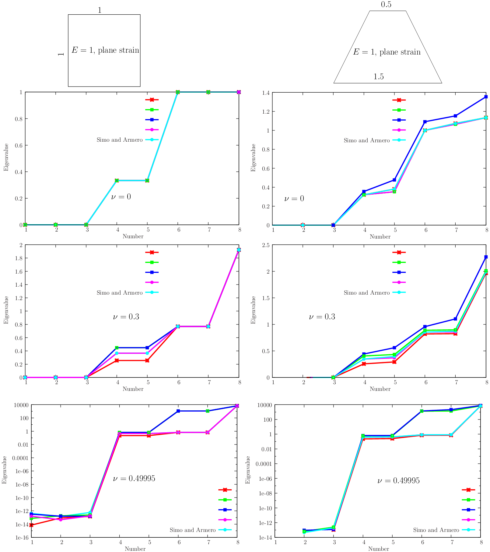
The inspection of the stiffness matrix eigenvalues for a single element is important to assess the differences between formulations. It is now known that different formulations can produce exactly the same results, and new derivations are often clones of long-standing ones (cf. [23]). Based on experience, we use four distinct configurations (square, trapezoidal, parallelogram and irregular) and three distinct Poisson coefficient values (ν = 0, ν = 0.3 and ν = 0.49995). Besides our formulation, we also inspect Simo and Armero Q1E4 element (cf. [50]), which entails the cost of additional degrees-of-freedom. Figures 1↓ and 2↓ summarize the results.
Figure 1 Eigenvalue results for the tested elements (α − δ) and Simo and Armero Q1E4. α and δ are used in SIMPLAS. (Square and trapezoid elements).
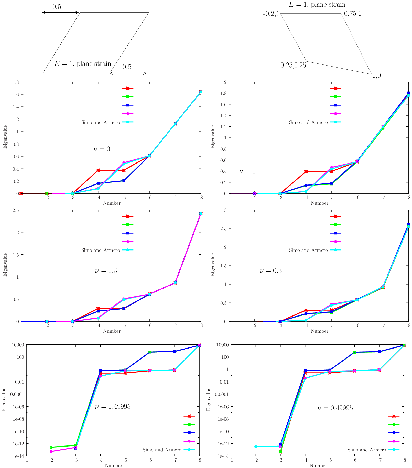
Figure 2 Eigenvalue results for the tested elements (α − δ) and Simo and Armero Q1E4. α and δ are used in SIMPLAS. (Parallelogram and distorted elements).
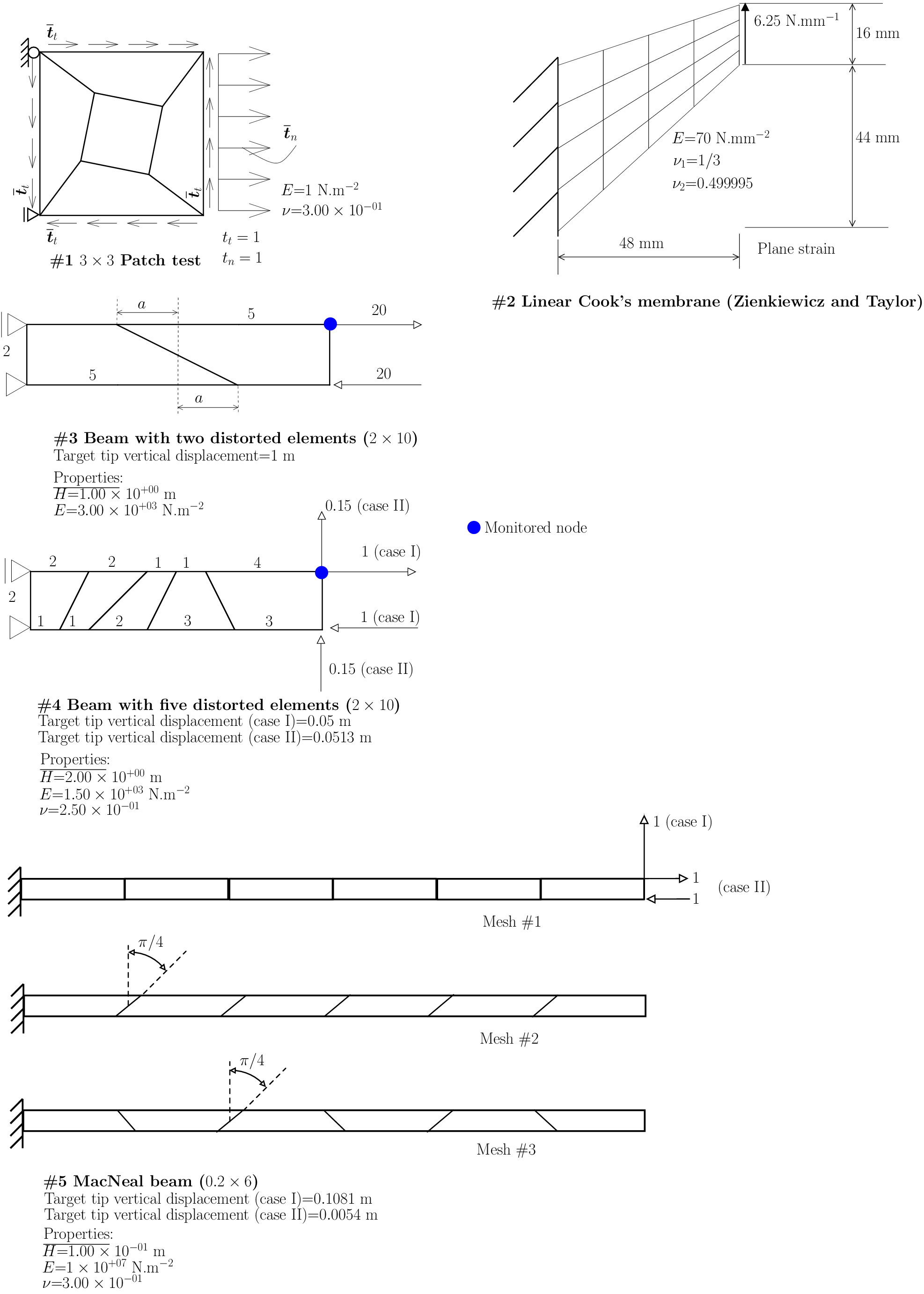
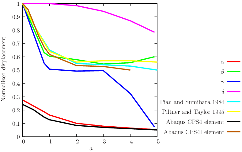
A set of five linear verification tests is depicted in Figure 3↓. Besides the Patch-test from T.J.R. Hughes textbook [27] (which is a requirement of SIMPLAS), we use the linear version of Cook’s membrane (as described in Zienkiewicz and Taylor [58]) to assess the behavior under bending combined with the incompressibility condition (Poisson coefficients ν1 = 1 ⁄ 3 and ν2 = 0.499995 are tested). Distortion locking (see, e.g. [23] for this nomenclature) is assessed by the beam problems with two and five distorted elements as well as the MacNeal slender beam with both parallel and trapezoid distortions (cf. [35]). We implemented the element by Simo and Armero formulation (cf. [50]) for comparison. We compare with elements from the literature that satisfy the Patch-test: Abaqus [1] CPS4 , CPS4I, CPE4H and CPE4I elements, Pian-Sumihara hybrid [37], Simo-Rifai enhanced assumed strain element (EAS) [52], Piltner-Taylor consistent EAS [38]. In addition, the recent “area-coordinate” quadrilaterals (e.g. [16]), presenting often exact solutions for benchmark problems, fail (cf. [39]) the Patch-test (the so-called weak Patch test was devised) and show grossly wrong solutions (cf. [39]) in problems other than the traditional benchmarks. Results for the Patch test and Cook’s membrane are shown in Figure 4↓ from which the following conclusions can be drawn:
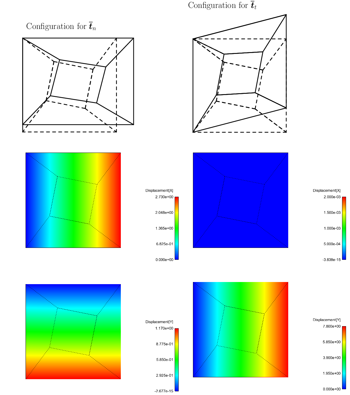
All proposed elements pass the Patch test exactly (with perfectly uniform stresses).
Element δ shows superior results when compared with Simo-Rifai element (see [58] for the results) and Pian and Sumihara. Abaqus CPE4I element reproduces the results of Simo-Rifai element.
Element α does not present locking in the incompressibility limit. Abaqus CPE4H element reproduces the results of α element, but requires an independent pressure.
Elements β and γ present locking in the incompressibility limit, and should therefore be avoided in general use.
Figure 3 Linear verification tests for plane quadrilaterals.
(a) Patch test results (all elements).
(b) ν = 1 ⁄ 3
(c) ν = 0.499995
Figure 4 Results for the Patch test and the linear Cook’s membrane.
(c) Normalized results for the MacNeal beam for two load cases and three mesh types.
Figure 5 Results for of the linear verification tests. Best results are highlighted.
Concerning the examples with distorted meshes, the following conclusions can be drawn:
For the two-element beam, element δ shows superior results to elements in the literature. Element α presents poor accuracy, similar to Abaqus CPS4. Element β shows results very similar to the Pian-Sumihara and Piltner-Taylor elements.
For the five-element beam, element δ shows excellent results, and with exception of the exactly integrated Korelc-Wriggers element [29] (not shown here since that version is limited to linear elastic problems), we could not find better results.
For the MacNeal beam, element δ is better in 3 out of 6 cases, tied with the Pian-Sumihara element.
Concluding, we found the element δ the only appropriate candidate for the use in linear and nonlinear problems when bending is present. Element α can also be used in problems where bending behavior is not essential. These two elements are used in SIMPLAS. The α is the default for plane strain and δ is the default for plane stress and optional for plane strain.
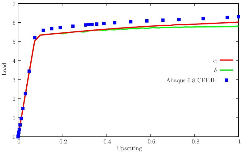
The well-known upsetting problem shows hourglassing patterns when the Q1E4 (the element of Simo and Armero [50]) is employed, see the paper by Crisfield et al.[19]. In that paper, the presence of hourglass instabilities was detected, despite the use of the 5 − point integration rule proposed by Simo, Armero and Taylor [49]. Therefore, it is an excellent candidate for inspection of the δ element in terms of hourglass patterns. Schonauer et al.[47] managed to reduce the reported instabilities and also reported the excessive coarseness of Crisfield’s mesh to model the shear band zone. The problem is defined in Figure 6↓ where consistent units are used. Pressure and effective plastic strain contour plots are shown, reproducing a diffuse shear band region. A comparison with Abaqus 6.8 element CPE4H is made for the upsetting/load curve (element CPE4I failed to converge at an early stage). Both proposed elements show slightly lower loads and present no signs of the hourglassing behavior reported by Crisfield.
Figure 6 Upsetting problem: definition, load/deflection results and contour plots for the δ element.
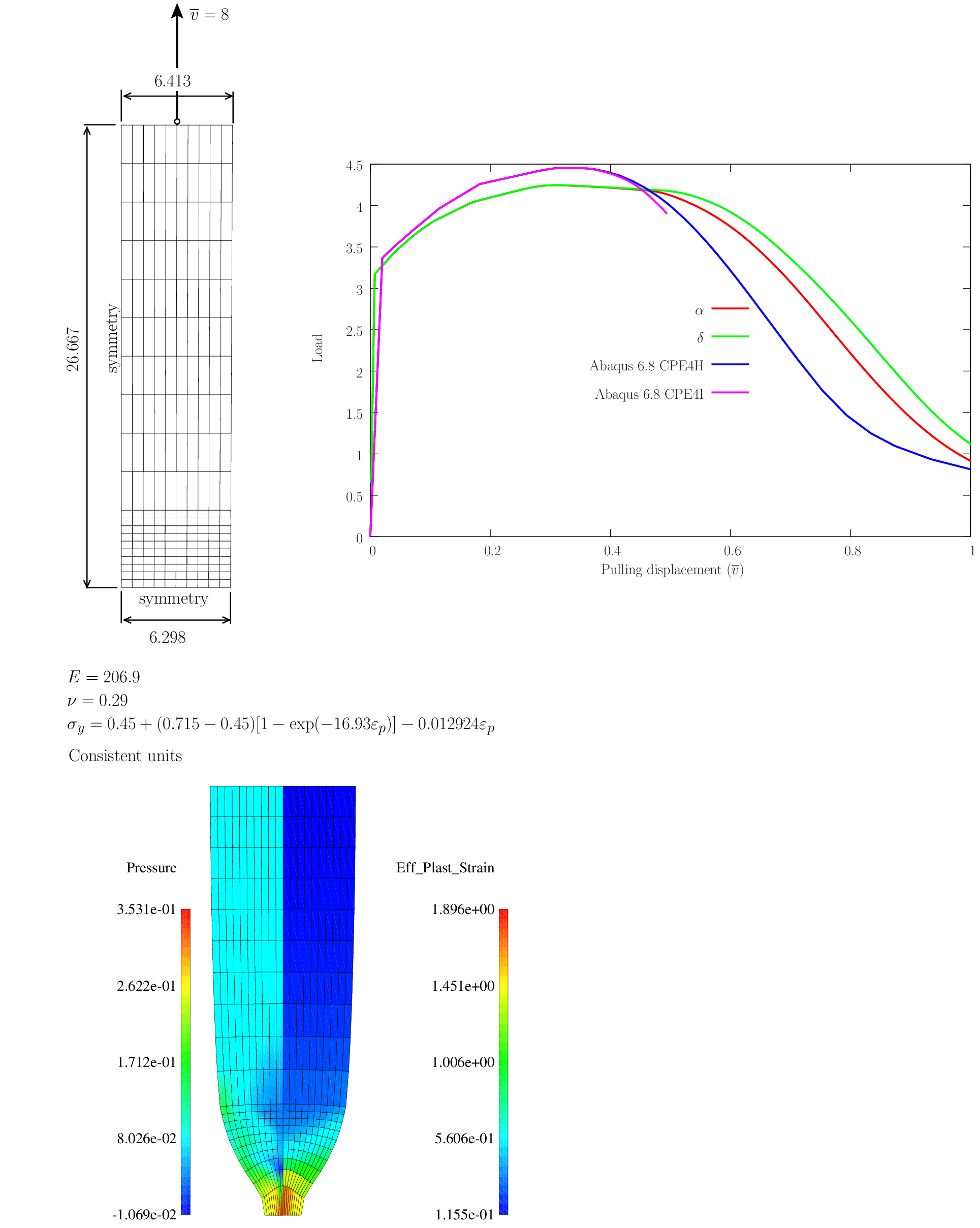
Element assessment in localization in a plane strain bar has been performed by Glaser and Armero [24]. A 200 element mesh is used, locally refined near the predictable necking zone (see Figure 7↓). This necking zone has a width 1.8% smaller than the pulling region. Taking advantage of symmetry, only one quarter of the bar is actually discretized. In Glaser and Armero, the context was the use of a special five-point quadrature aimed at attenuating the hourglass instabilities present in the original Q1E4 element. The test and results for elements α and δ are depicted in Figure 7↓. No hourglass was observed and results were compared with Abaqus 6.8 CPE4H and CPE4I elements. It is noticeable that the latter failed to converge. We can observe that our elements α and δ present somehow delayed localization when compared with Abaqus, but peak load is lower.
Figure 7 Plane strain localization problem: relevant data and effective strain and pressure contour plots.
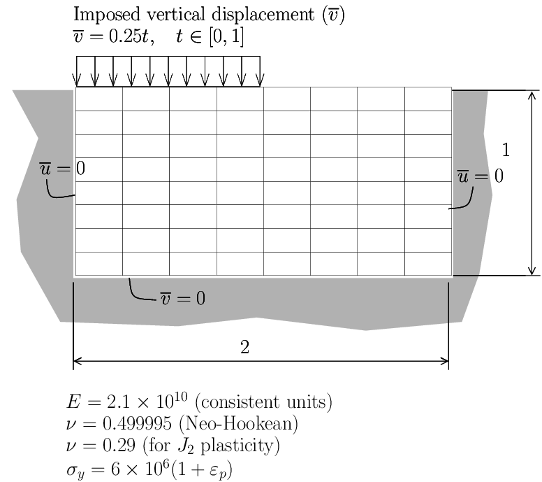
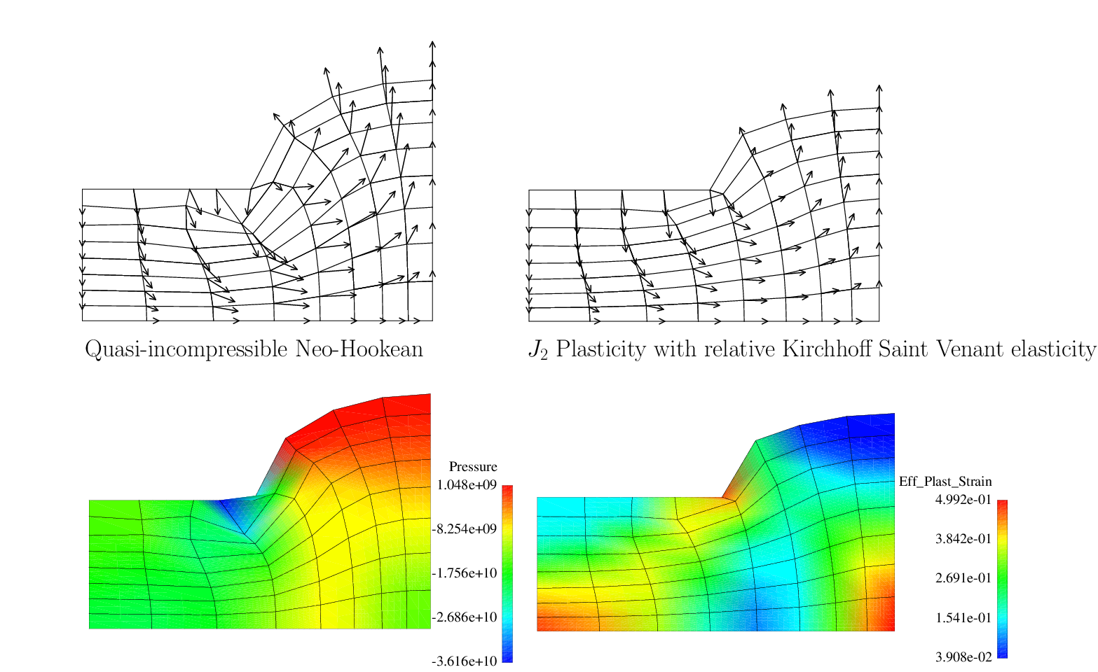
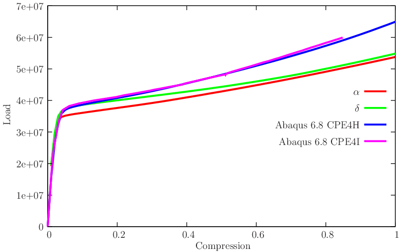
Two classical versions of the asymmetric block indentation problem inspired by Crisfield work (cf. [19]) are assessed here: one with quasi-incompressibility elasticity (Quasi-incompressible Neo-Hookean material) and another with J2 plasticity/relative Kirchhoff Saint Venant elasticity. The problem data is shown in Figure 8↓. Results for both versions are shown in Figure 9↓ where the displacement vector maps and contour plots are shown. Conclusions are drawn from this test:
No hourglass patterns are present in the results;
Both elements α and δ are immune to locking in the incompressible limit;
Results are less stiff than both elements CPE4H and CPE4I in Abaqus 6.8 (see also the convergence curve 10↓);
Element CPE4I fails to finish the run due to lack of convergence in the Newton iteration.
Figure 8 Block indentation: geometry and mesh, boundary conditions and material properties.
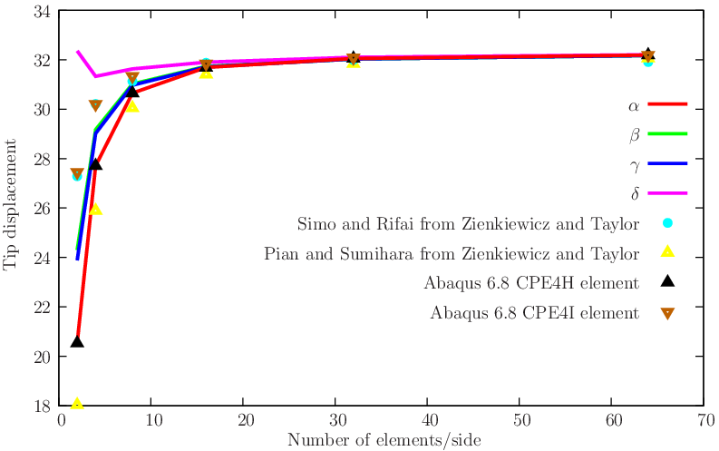
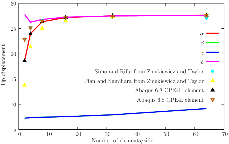
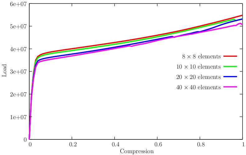
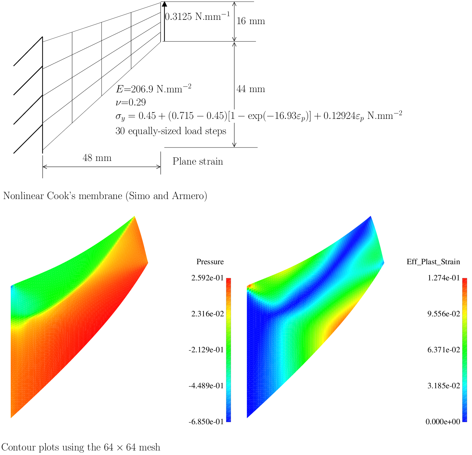
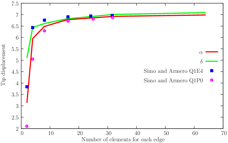
We use a nonlinear version of the Cook’s membrane shown in Figure 3↑ with J2 plasticity as discussed by Simo and Armero [50]. Other comparisons were made by César de Sá, Areias and Jorge (cf. [17]) where improved results were shown. We here are concerned with the convergence of the α and δ elements with the number of elements, as well as oscillations in the pressure distribution for the δ element. Figure 11↓ describes the problem and shows the contour plots. Neither hourglassing nor pressure oscillations are present. In terms of convergence of the tip displacement, the results by Simo and Armero are shown for comparison in Figure 12↓ where the excellent behavior of the δ element can be observed.
Figure 11 Elasto-plastic finite strain Cook’s membrane (cf. [50]). Problem definition, pressure and effective plastic strain contour plots for the 64 × 64 element mesh.
Figure 12 Convergence of the elasto-plastic finite strain Cook’s membrane.
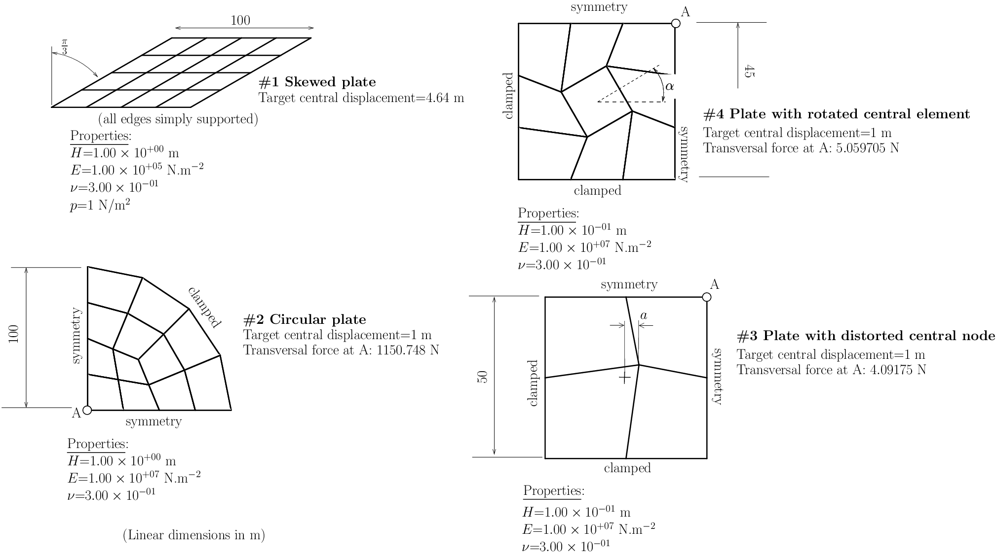
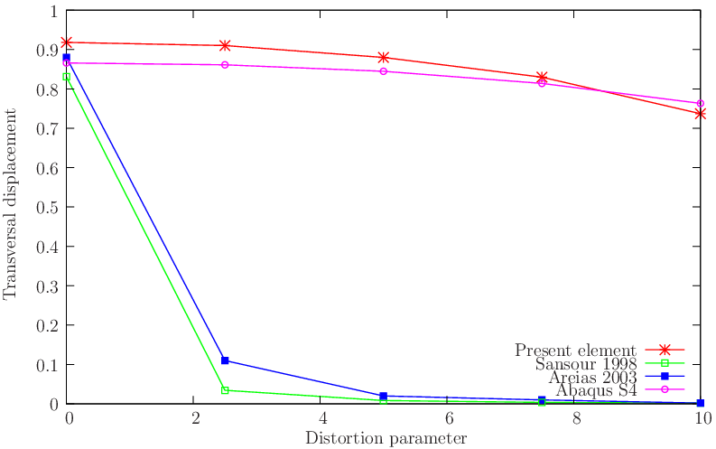
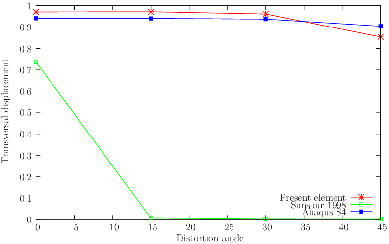
Plate bending tests for verifying the implementation in the linear case are detailed in Figure 13↓ (where the relevant data for the tests is shown) and in Figures 14↓ and 15↓ (comparisons with results from the literature). In Figure 14↓ comparisons are shown with the results presented in references [37, 12, 4, 33, 38, 54, 32, 44, 7] and the Abaqus S4 element. In all examples we use standard Gaussian quadrature with 2 × 2 Gauss points in the plane and 2 points along the thickness. Noting that although no enrichment of the displacement and rotation fields are performed, the present element is competitive with the best available formulations.
Figure 13 Linear plate bending tests: relevant data and target values for monitored nodes.
(a) Skewed plate (#1)
(b) Circular plate (#2)
(c) Square plate with distortion (#3)
Figure 14 Verification tests: linear plate problems: comparison with alternative formulations (problems #1, #2 and #3).
Figure 15 Verification tests: Square plate with angle distortion (#4).
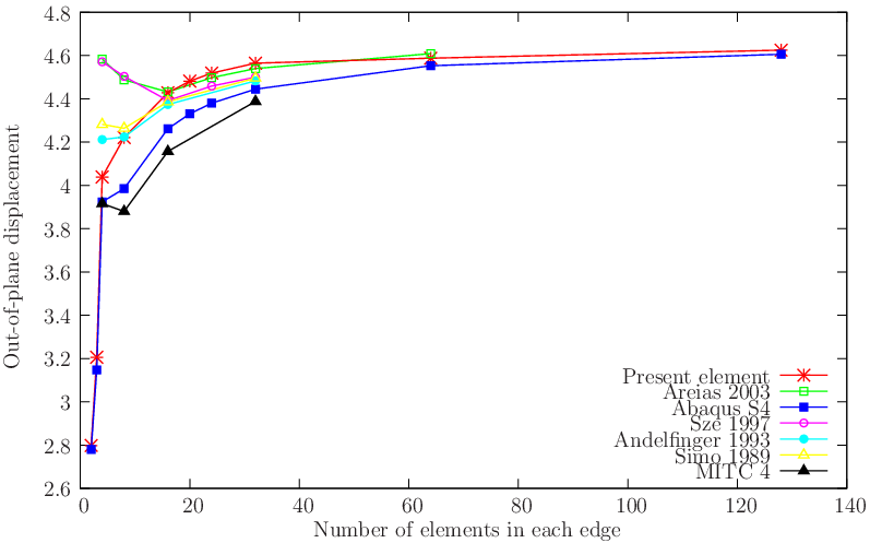
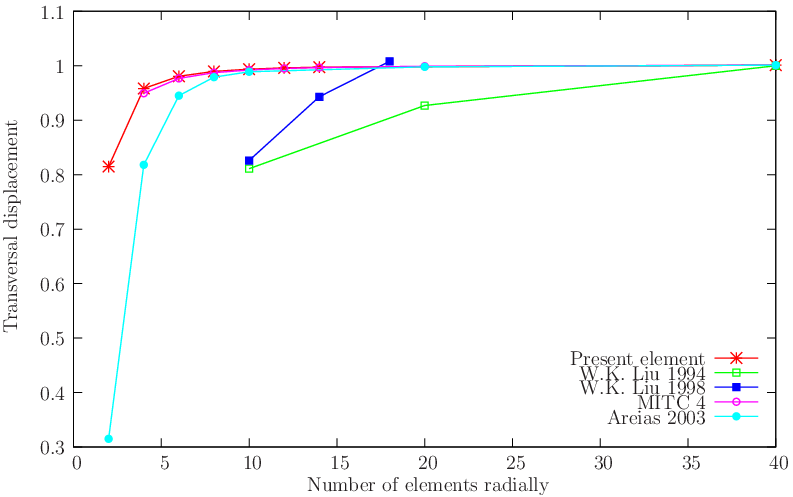
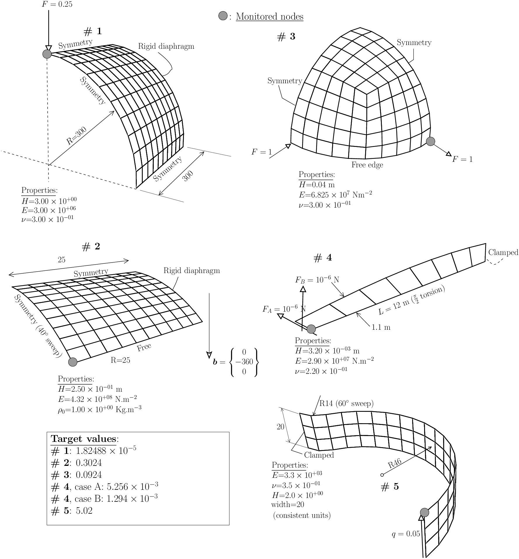
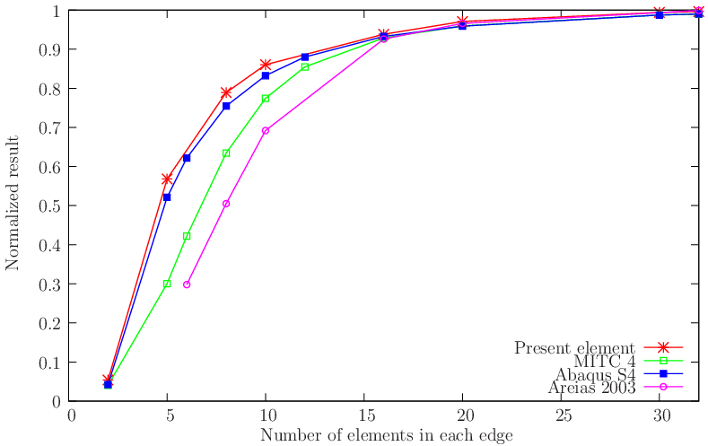
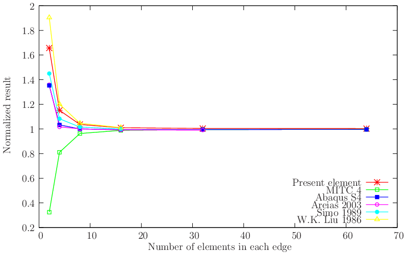
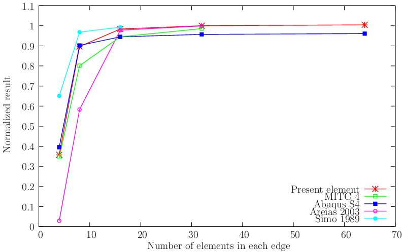
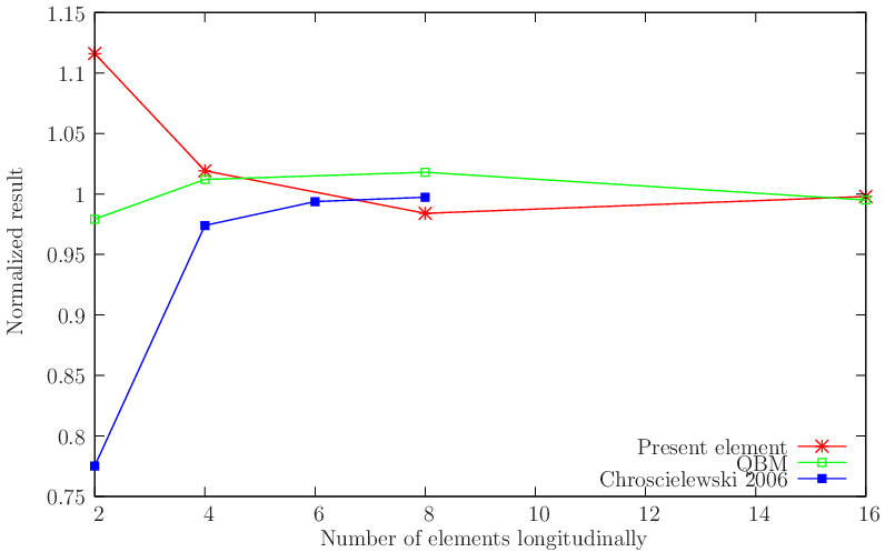
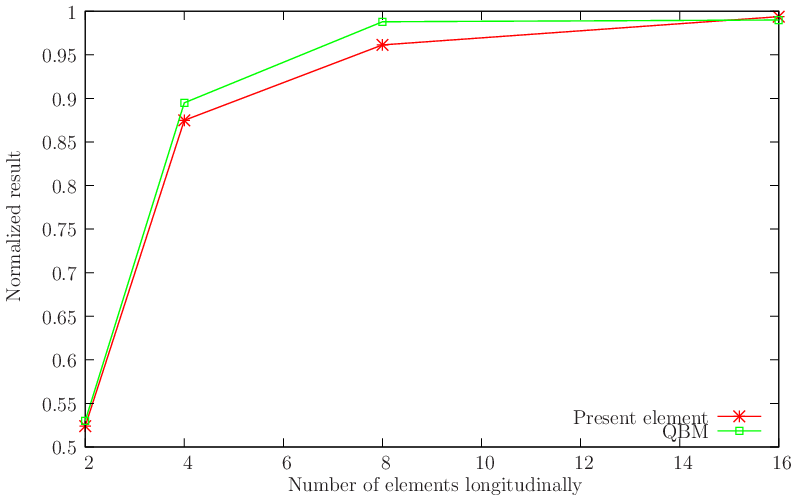
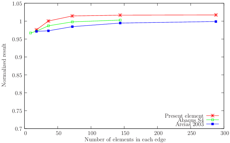
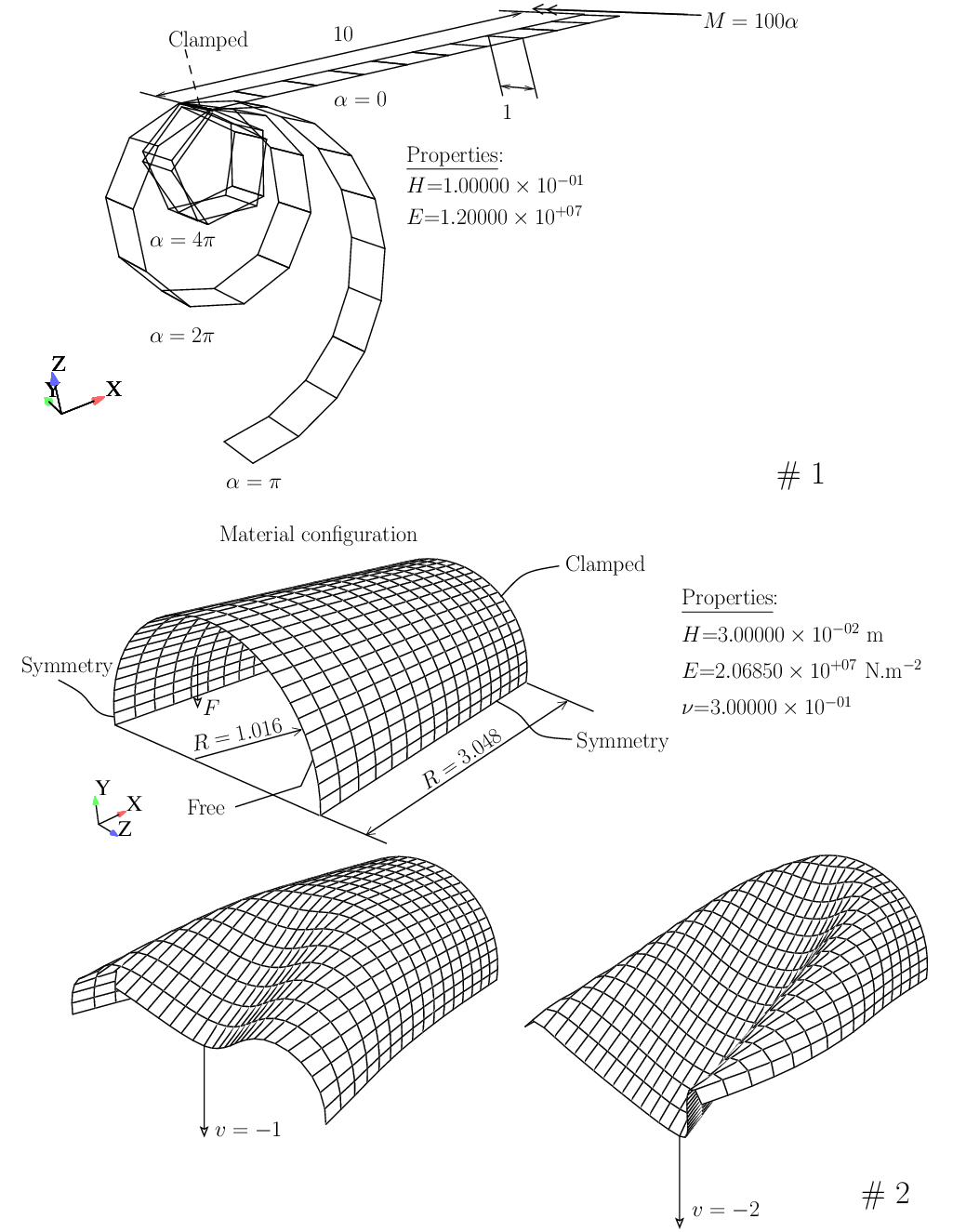
Linear shell tests are important for assessing competitiveness in both linear and nonlinear codes. Results in nonlinear problems are conditioned by the inherent linear formulation. However, due to the presence of interfering constitutive laws, stress integration and other interfering ingredients, results from nonlinear problems are seldom conclusive concerning the accuracy of the underlying interpolation approach. Therefore, we first focus on the five classical shell tests depicted in Figure 16↓. This Figure contains the relevant data. Results are compared with known element formulations in Figures 17↓ and 18↓. Test #1 is the well-known pinched cylinder problem (a reference value of 1.82488 × 10 − 5 m is used in the normalization, in agreement with Simo, Fox and Rifai [51]). For this test, results shown in Figure 17↓ attest the good performance of the present element. Test #2 is the Scordelis-Lo roof (see [35]) in which our element was found to have similar performance to the S4 element from Abaqus. Our implementation of Dvorkin and Bathe [20] MITC4 element results in slightly stiffer results in both tests #1 and #2. Test #3 is the closed pinched hemisphere [A] [A] The open 18○ variant does not provide additional information. with a target value of the radial displacement of 0.0924[51]. In this test, we found that our element converges faster than the S4 and MITC4 elements for coarse meshes. The test #4 is the so-called twisted beam and it has been adopted in many references with several variants. Our variant is the most demanding (with a thickness of 0.0032 m) and was proposed by Belytschko and Wong [13]. Two load cases are inspected, as indicated in Figure 16↓. Excellent results were obtained by the present formulation in case A. Test #5 is the so-called Raasch’s hook (cf. [48]) and involves bending and torsion. The target value adopted here is 5.02 consistent units (also employed in the first Author’s Ph.D. thesis and the Abaqus/Standard benchmark suite). Considered meshes are (elements × elements): 1 × 9, 3 × 18 , 5 × 36, 10 × 72, 20 × 144 and 40 × 288 elements. Results appear somehow worse than Abaqus S4 but the target value is well approximated by the present element. An inspection shows very good results for coarse meshes. The present results are better than the previous high-performance element HIS (cf. [7]) and QBM (cf. [10]). Overall, SIMPLAS shows one of the best performing elements four-node shell elements.
Figure 16 Linear shell tests: relevant data and target values for monitored nodes.
(a) Cylinder (#1)
(b) Scordelis-Lo roof (#2)
(c) Sphere (#3)
Figure 17 Linear shell tests: results for problems #1, #2 and #3.
(a) Twisted beam (#4), case A
(b) Twisted beam (#4), case B
(c) Raasch’s hook (#5)
Figure 18 Linear shell tests: results for twisted beam (#4) and Raasch’s hook (#5).
2.3 Geometrically and materially nonlinear problems
This section shows the applicability to classical nonlinear problems and thecapabilities of the formulation, specifically:
Higher levels of load and displacement factors than previously published.
Large load steps and consistency of results between different load steps.
Asymptotically quadratic rate of convergence for the Newton method.
Nonlinear problems are shown in two sets: finite-displacement elastic problems (specifically hypoelastic) and finite strain plasticity problems.
Figure 19 Finite-displacement problems: relevant data and target values for monitored nodes.
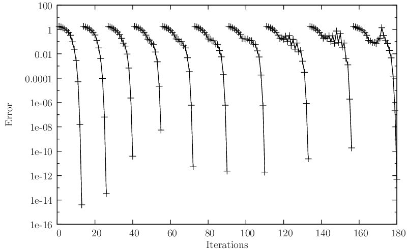
Two classical geometrically non-linear problems are solved, with the corresponding data summarized in Figure 19↑. Results for the clamped pinched cylinder (cf. [22]) are shown in Figures 20↓ and 21↓. These attest the robustness of the proposed formulation. Specifically, Newton-Raphson convergence is asymptotically quadratic (cf. Figure 21↓) since an exact linearization is performed [B] [B] We restrict the Newton step size to avoid iterating outside the convergence radius (5% of the geometrical dimensions for the displacement step and 0.05 Radians for the rotation degrees-of-freedom)..
Figure 20 Clamped pinched cylinder: specific results compared with reference numerical solution [22].
Figure 21 Error values vs. iterations for the 10 step case (clamped pinched cylinder).
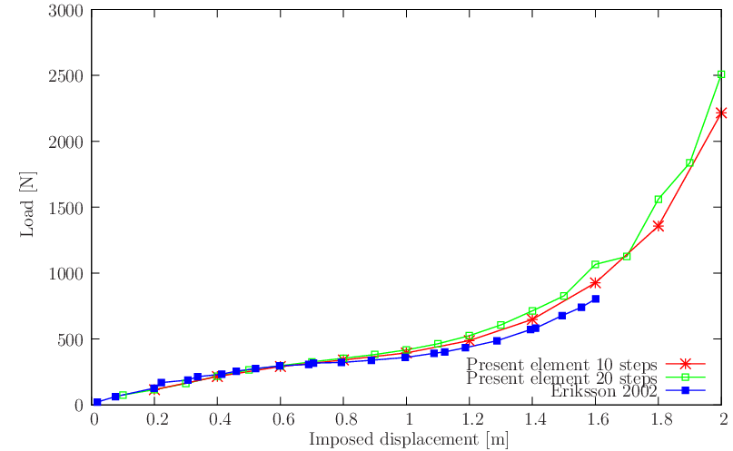
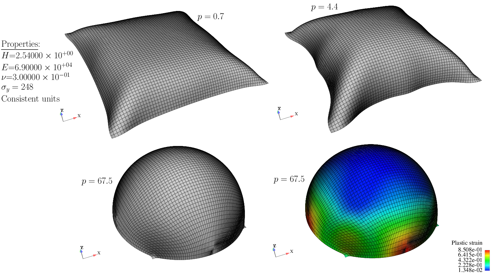
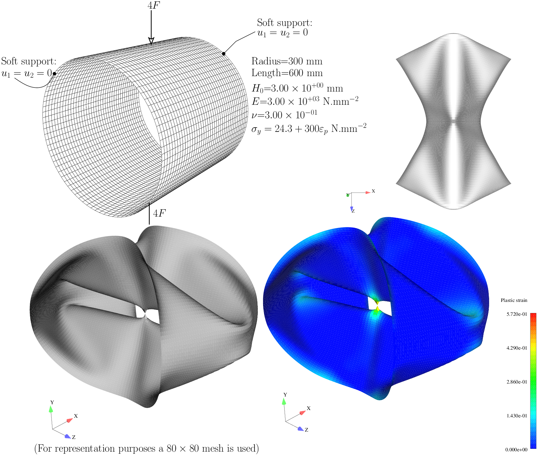
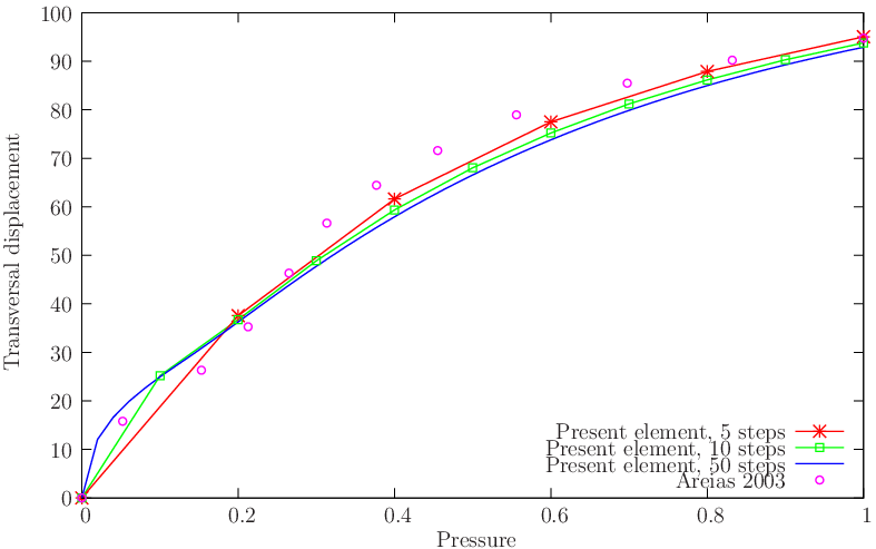
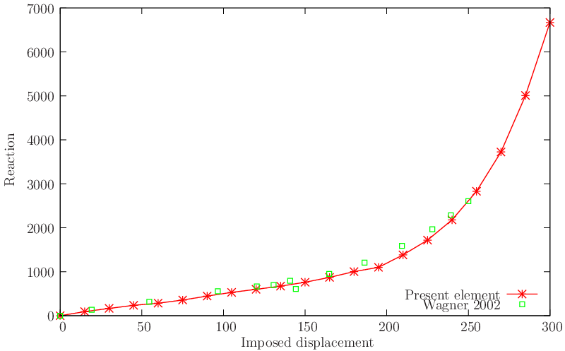
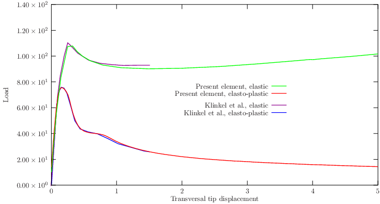
Two finite strain plasticity problems are solved using our recent algorithm (cf. [9]): the elasto-plastic plate under deformation-dependent pressure and the pinched cylinder (both with plane stress von-Mises plasticity). Relevant data and deformed meshes (and contour plots) for these problems are shown in Figure 22↓. The plate under pressure was described by Hauptmann et al.[26] and further inspected in [7]. It consists of a plate with dimensions 508 × 508 × 2.54 consistent units. Elasticity modulus is E = 6.9 × 10⁴ consistent units, Poisson coefficient ν = 0.3 and the yield stress is σy = 248 consistent units. One-fourth of the plate is analyzed with 32 × 32 elements with a sequence of deformed meshes and the effective plastic strain contour plot shown in Sub-Figure a↓. Results are presented in Figure 23↓. As for the other problem (pinched cylinder test with soft support), it is depicted in Sub-Figure b↓ and was also tested in [7]. It consists of a cylinder with 300 mm of radius, with E = 3000 MPa, ν = 0.3 and a linear hardening law: σy = 24.3 + 300εp MPa. Load-deflection results for the 16 × 16 are shown in Figure 23↓, are close to the ones by Wagner, Klinkel and Gruttmann [56] for high values of pinching displacement.
(a) Square plate under deformation-dependent pressure: data and sequence of deformed meshes.
Figure 22 Finite strain plasticity problems: relevant data and results.
Figure 23 Finite strain plasticity problems: load/deflection results compared with [7] and [56].
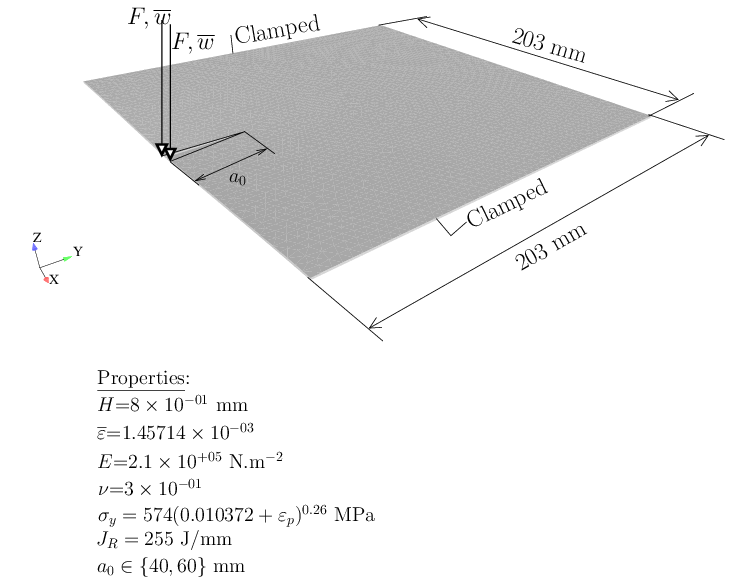
Figure 24 Muscat-Fenech and Atkins plate (cf. [36]). Relevant data. The Sutton criterion is used to determine the crack path (cf. [34]).
(a) Effective plastic strain contour plot
(b) Load-deflection curve
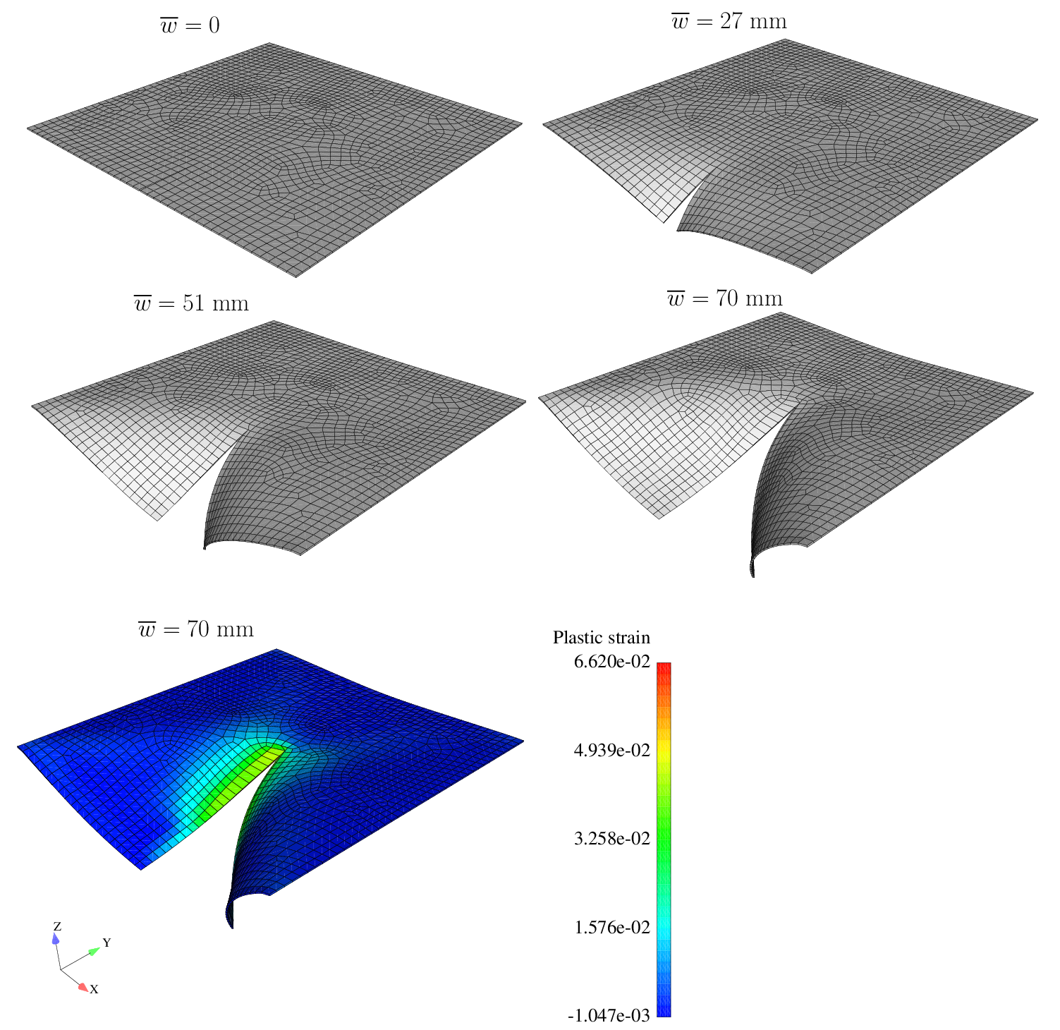
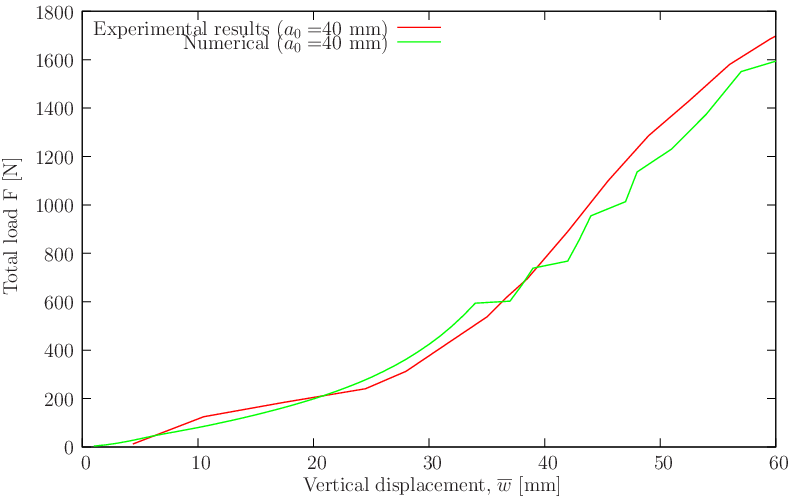
Figure 25 Muscat-Fenech and Atkins plate (cf. [36]) for a0 = 40 mm. Deformed meshes and effective plastic strain contour plot are shown. Also shown is the load-deflection curve.
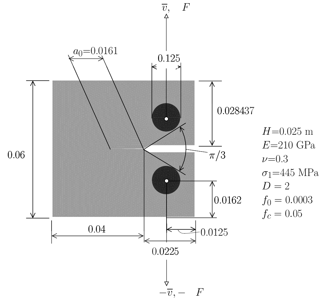
The Muscat-Fenech and Atkins plate (studied by these Authors and reported in [36]) was already tested numerically using the extended finite element method (XFEM) in Areias and Belytschko (see [5]). It was found that reasonable results are obtained combining J2 plasticity with a cohesive law. Only a slight deviation from the experiments was observed near the end of the analysis. Relevant data for this problem is shown in Figure 24↑. A pre-cracked steel plate is subject to two vertical forces F as indicated in that Figure. The crack advance criterion is the principal maximum strain (ε = 1.45714 × 10 − 3) corresponding to the maximum normal stress of 306 MPa. A fracture energy of JR = 255 N/m is used, the upper limit of what is reported in [36]. The Sutton criterion [34] is used for the crack path. Results are shown in Figure 25↑ where reasonable agreement can be observed.
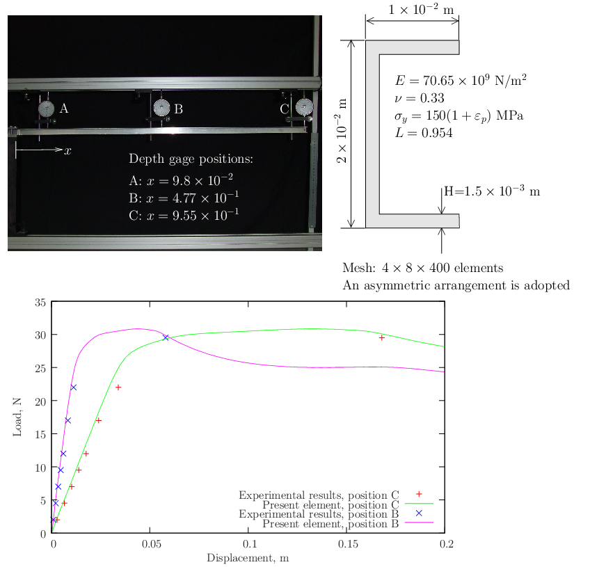
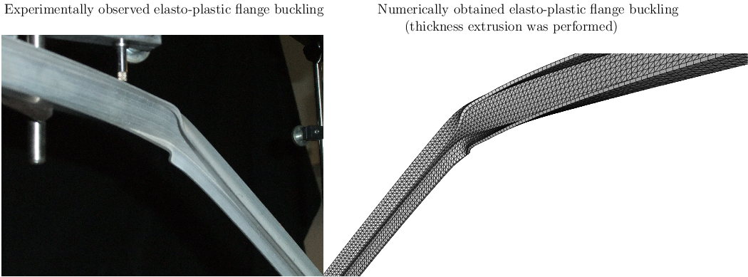
A slender beam with a C profile made from ductile aluminum was clamped to our laboratory frame as shown in Figure 26↓. The loading strategy was very simple: 2 N, 2.5 N and 5 N disks were added to a hook hanged at a drilling in the beam and depth comparators were set above the beam. We employed a non-linear least-square code to determine the elasticity modulus. The hardening law was, in contrast, estimated by trial-and-error. Elasto-plastic buckling occurs at the flanges as shown in Figure 27↓. Comparative results for the proposed element are also shown in Figure 26↓.
Figure 26 Cantilever beam: experimental arrangement, cross-section dimensions and material properties.
Figure 27 Cantilever beam: comparative pictures of the elasto-plastic buckling of the flange and numerical prediction.
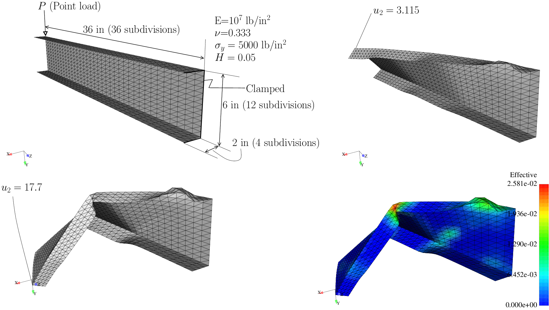
The predictive capability was found to be very good. The channel section cantilever beam by Eberlein and Wriggers [21] is reproduced here. Recently, Klinkel, Gruttmann and Wagner [28] tested this problem with a hybrid quadrilateral, although to a lower deformation than in the original paper. Relevant data is shown in Figure 28↓ where deformed and undeformed meshes are shown for a sequence of steps. We subdivide each quadrilateral element in [28] with four triangles. The load-deflection results are shown in Figure 29↓ and compared with reference [28]. Reasonable agreement with the reported results in [28] can be observed.
Figure 28 Channel section cantilever beam: geometry, boundary conditions and sequence of deformed meshes. Thickness-averaged effective plastic strain is shown.
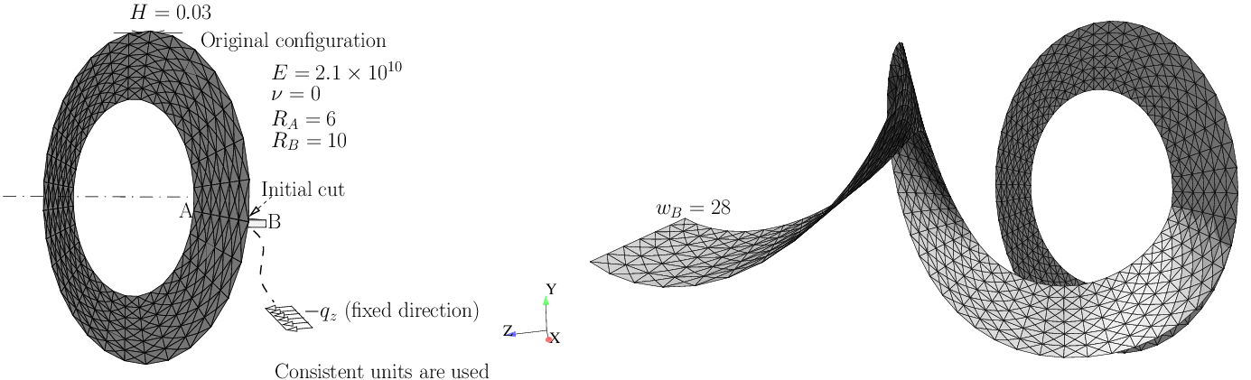
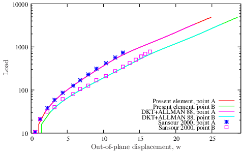
The first smooth plate is the ring test first proposed by Başar and Ding [11] to test formulations for finite rotations in shells. The relevant geometry, boundary conditions and elastic properties are depicted in Figure 30↓. We extend the ring up to 28 consistent units. Figure 30↓ depicts this extension. A comparison with the results by Sansour et al.[45] is also shown in Figure 31↓. We can observe that with our method we attain a higher value of ring extension and slightly more flexible results. Between the present element and a combination of DKT and Allman’s element, no differences were noted, in contrast with what was observed in the linear tests.
Figure 30 Ring test by Başar and Ding [11]. Consistent units are used.
Figure 31 Ring test: comparison with the results by Sansour et al.[45]
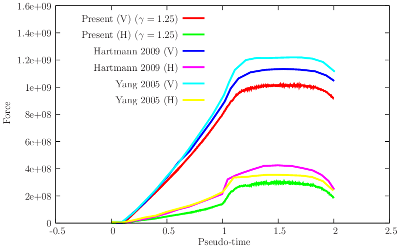
This benchmark has been used to advocate the use of mortar discretizations in contact problems, cf. Yang, Laursen and Meng [57]. We solve the ironing problem introduced by to support the use of mortar contact elements. Figure 32↓ shows the relevant geometric and constitutive data, agreeing with the references [57] and [25]. We compare the present approach with the results of these References in Figure 33↓. Differences exist in the magnitude of forces, and we concluded that this is due to the continuum finite element technology. We use finite strain B-Bar elements (cf. [53]), known to be more compliant than the standard Q4 isoparametric elements.
Figure 32 Ironing problem: relevant data and deformed mesh snapshots.
Figure 33 Ironing problem: results for the load in terms of pseudo-time, compared with the values reported by Yang et al.[57] and Hartmann et al.[25].
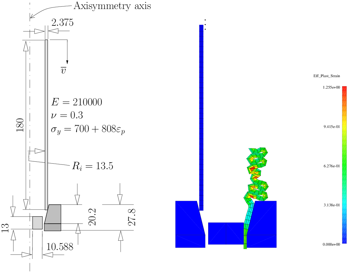
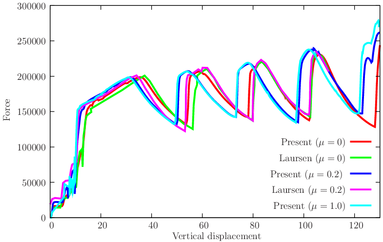
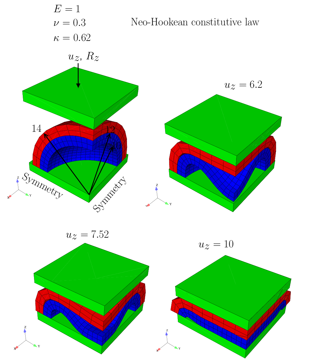
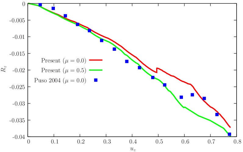
This classical elasto-plastic axisymmetric problem, relevant for crashworthiness studies was introduced by Laursen (cf. [31]). In his work, Laursen used the operator split method with the augmented Lagrangian method to solve the crushing of a cylinder. He used μ = 0 and μ = 0.2 to assess the implementation. We here reproduce this problem, and solve it with μ = 0, μ = 0.2 and μ = 1. We use the consistent elasto-plastic integration algorithm discussed in [9]. Results are shown in Figures 34↓ and 35↓ allow the following conclusions:
For μ = 0, our algorithm predicts the post-buckling behavior earlier than Laursen. In addition, higher imposed displacements are possible with our algorithm. We note that a slightly lower penetration in the rigid fixture when compared with Laursen.
For μ = 0.2, our algorithm produces very similar results to the ones reported by Laursen.
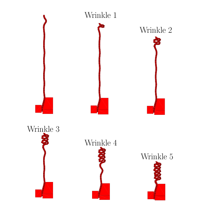
We also tested μ = 1 with visible differences with respect to the case μ = 0.2 in the fifth wrinkle.
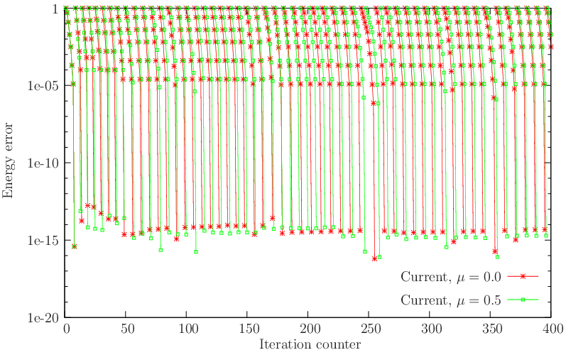
We also show, for μ = 0.2, the error evolution as a function of iteration count in Figure 45↓.
Figure 34 Post buckling of an elasto-plastic cylinder. A picture corresponding to the 5 wrinkles (cf. 4 were reported by Laursen [31]) is also shown.
Figure 35 Post buckling of an elasto-plastic cylinder: compression/reaction results. A comparison with the results reported by Laursen [31] is performed.
Figure 36 Post buckling of an elasto-plastic cylinder: sequence of wrinkle formation.
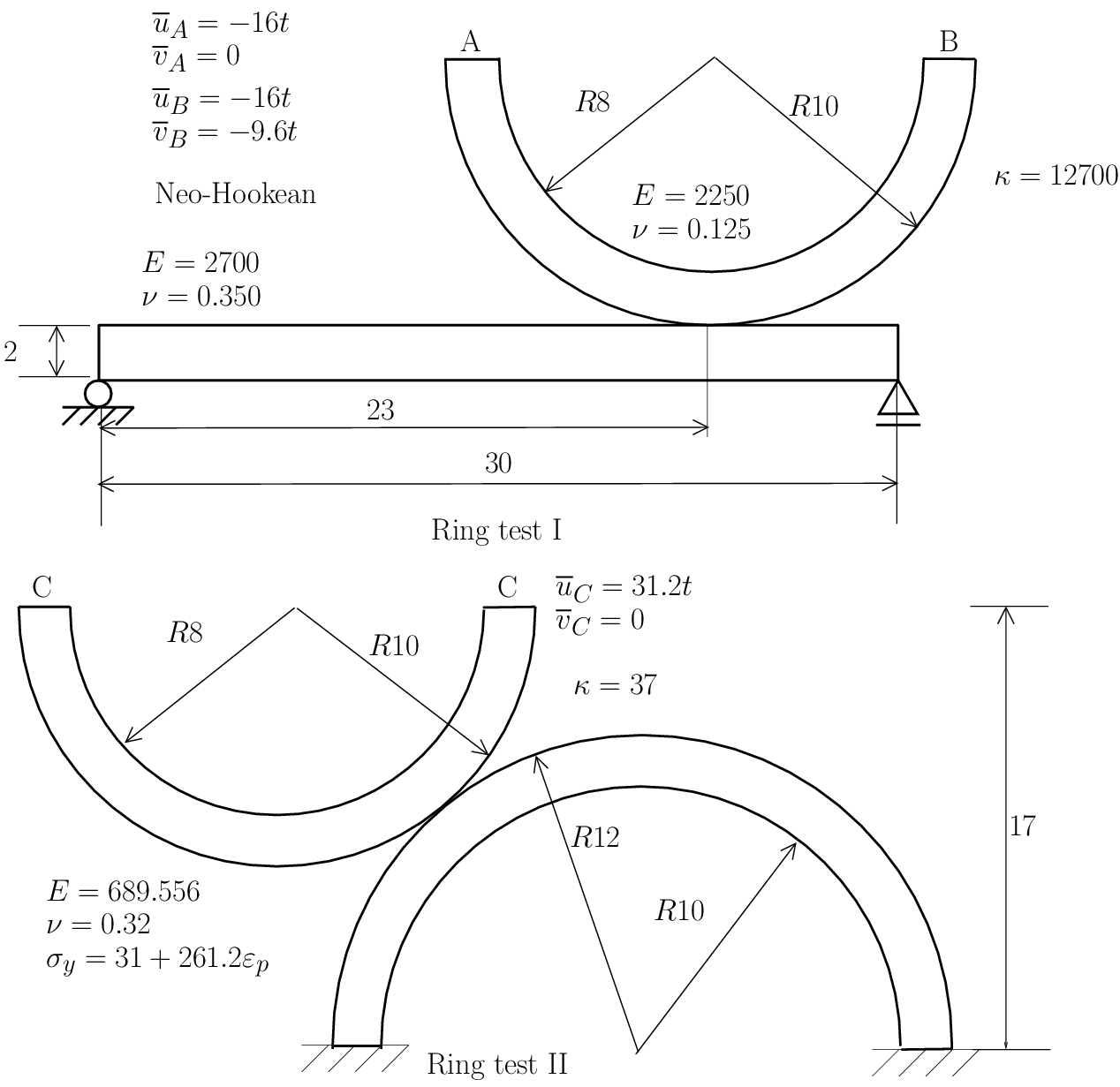
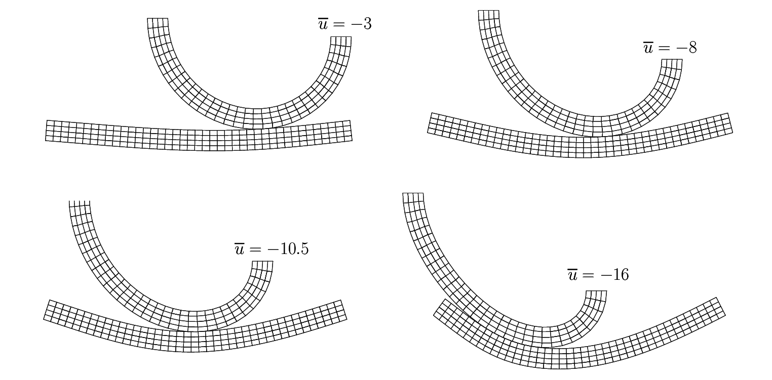
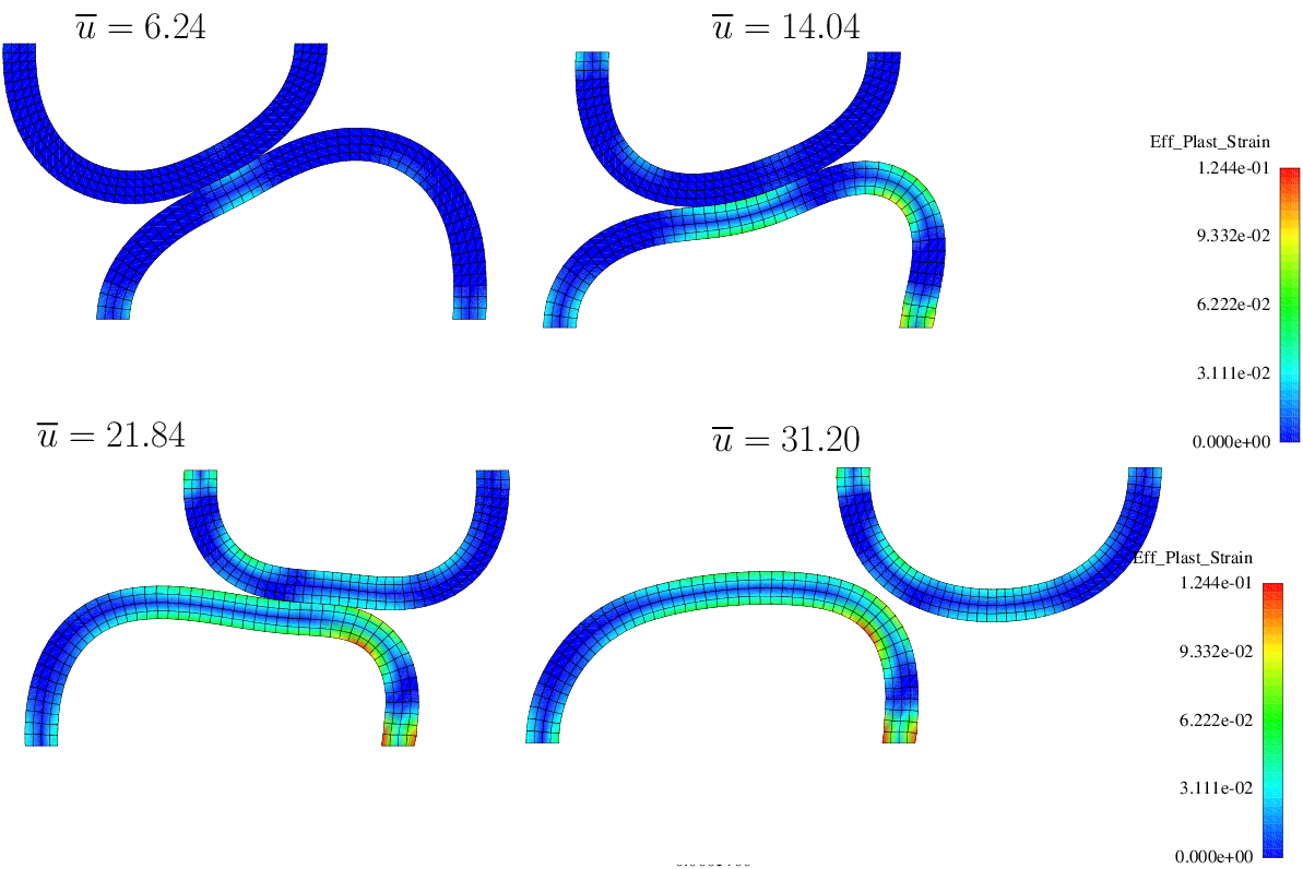
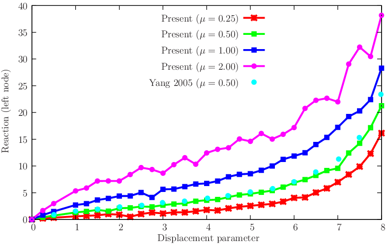
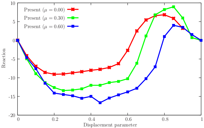
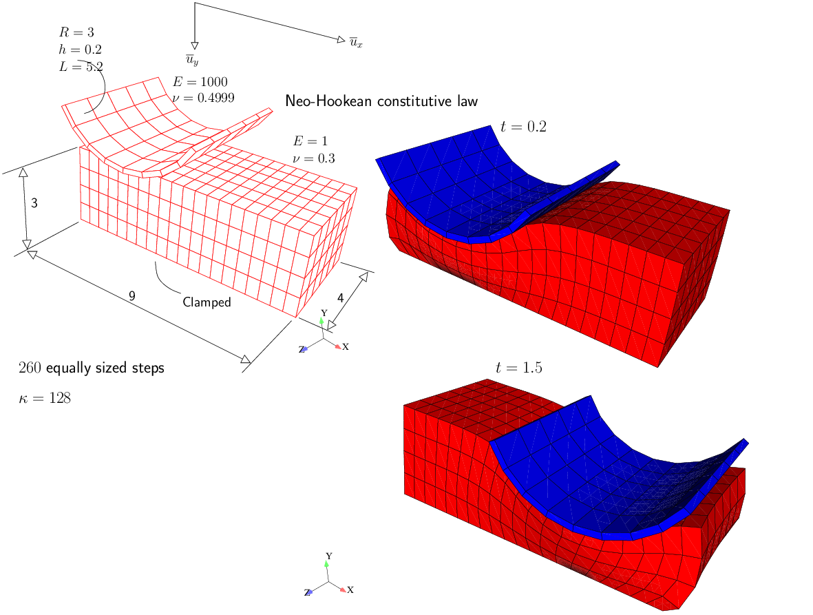
These are other examples typically adopted within the mortar formulation contexts (cf. Yang et al.[57]). We here use these examples to assess the (quadratic) cone projection method for problems typically solved by mortar discretization techniques. Figure 37↓ shows the relevant data for the two tests. In test I, a Neo-Hookean constitutive law is used and in test II J2 plasticity is used with our recently proposed algorithm [9]. A sequence of results produced by the proposed algorithm is shown in Figure 38↓ for both tests. The effective plastic strain contour plot for test II is very similar to the one obtained by Yang et al.[57]. The evolution of reactions is also compared with published results in Figure 39↓. Good agreement with the mortar technique can be observed. We also show results for μ = 1 and μ = 2 and for these high values, slight oscillations appear.
Figure 37 Geometrical, boundary conditions and constitutive data for the ring frictional tests.
(a) Ring test I: sequence of deformed meshes.
(b) Ring test II: contour plots for effective plastic strain.
Figure 38 Sequence of configurations for the two ring tests.
(a) Ring test I.
(b) Ring test II.
Figure 39 Results for the two frictional tests involving rings.
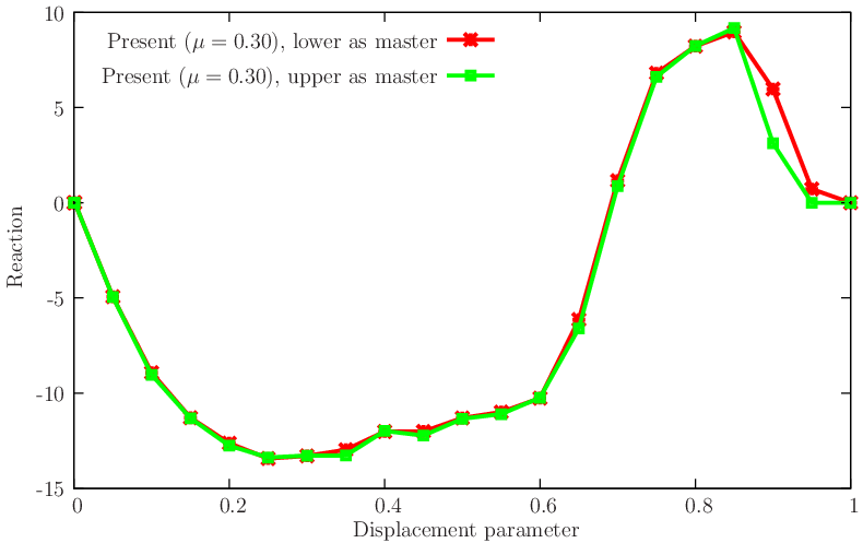
The effect of choosing the upper or lower surface as master is shown in Figure 40↓ where it can be observed that only the end values differ.
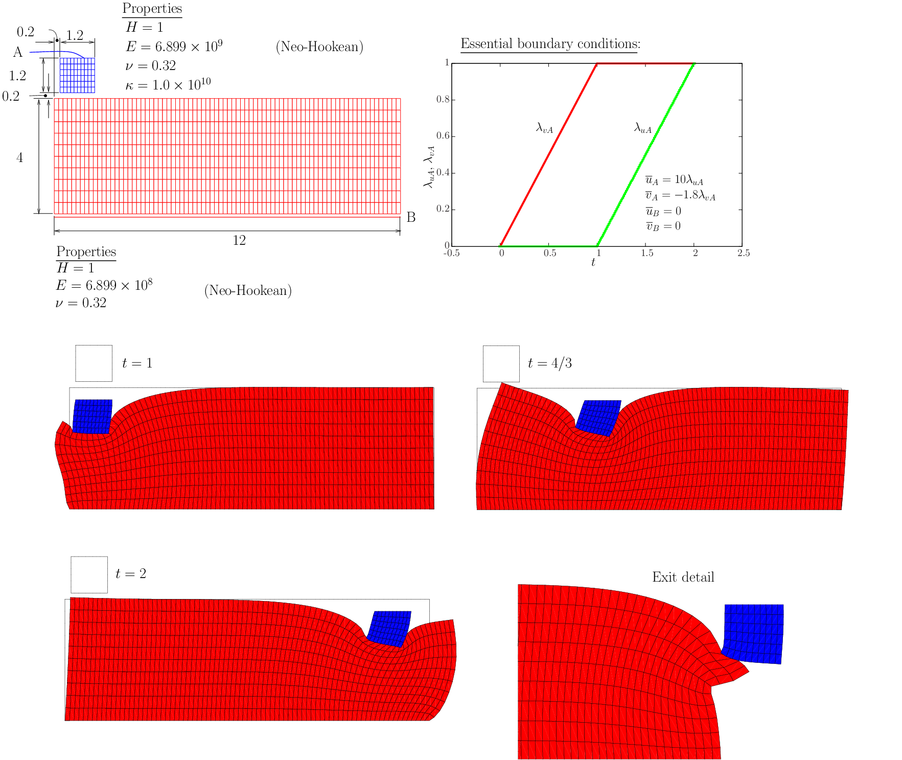
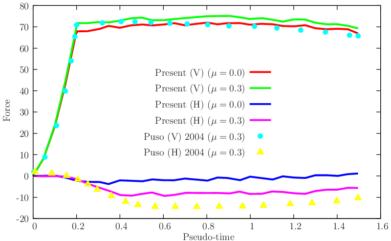
We reproduce the problem of Puso and Laursen [41] who detected locking with node-to-segment approach. Relevant problem data is shown in Figure 41↓. Two stages of displacement of the deformable die (whose center is located at 2.5 units from the slab end) are used: in the first stage, t ∈ [0, 0.2] the die lowers into the slab a total of 1.4 units. In the second stage, t ∈ ]0.2, 1.5], the die moves 4 units in the longitudinal direction of the slab. Reaction results are shown in Figure 42↓ where good agreement with Reference [41] can be observed for the normal reactions. However, the tangential reactions are slightly lower in magnitude for our case.
Figure 41 3D ironing problem: relevant data and deformed meshes.
Figure 42 Reactions and comparison with the results of Puso and Laursen (cf. [41]).
The paper by Puso and Laursen [40] presents the concentric sphere problem indicating premature failure of the node-to-face algorithm (even for the frictionless case). Meshes are purposively incompatible to force gap discontinuities to occur during sliding of sphere faces. Figure 43↓ presents the relevant data for this problem (we explicitly represent the two obstacles). We solve this problem to a slightly lower imposed displacement and inspect the effect of friction in the interface between the two hollow spheres (contact with the obstacles has zero friction coefficient). Note that, in [40], no friction was present. Figure 44↓ shows the reaction results, compared with the values reported by Puso and Laursen [40]. The evolution of the energy error during Newton iteration is shown in Figure 45↓.
Figure 43 Compressed concentric spheres: relevant data and sequence of configurations.
Figure 44 Compressed concentric spheres: displacement/reaction results, compared with [40].
Figure 45 Compressed concentric spheres: Evolution of energy error in Newton iteration for μ = 0.0 and μ = 0.5 (scaled to give 1 for each first iteration). First 400 iterations (with history updating counting as an extra iteration) are shown.
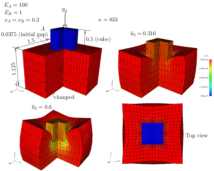
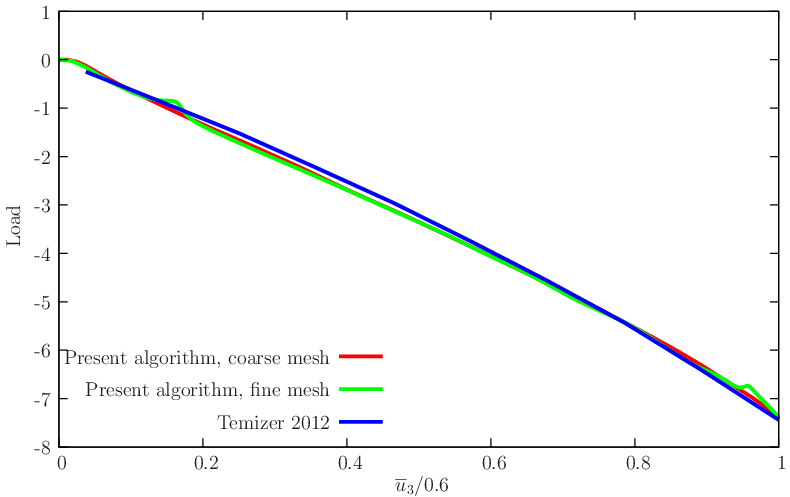
We now reproduce the benchmark proposed by Temizer [55] which introduces sharp corners and edges in 3D and finite strains (with the neo-Hookean constitutive model). We represent two compressed blocks using one-quarter of the geometry, as depicted in Figure 46↓. Temizer uses two distinct meshes (a coarse mesh with 5 × 5 × 3 elements for the lower block and a fine mesh with 8 × 8 × 4 elements). The present method requires a finer mesh so that severe spurious inter-penetration (edge/edge crossing) does not occur. Often, contact problems are apparently successfully solved with the node-to-face algorithm but in close inspection there are large edge crossing or wrong target face selections. Also, this fact is known to cause oscillations in the load response. Although there are ad-hoc remedies to this, we usually employ two sufficiently refined meshes. Our coarser mesh consists of:
Top block with 6 × 6 × 2 elements.
Bottom block with 9 × 9 × 5 elements.
A finer mesh with a bottom block containing a 12 × 12 × 8 arrangement is also adopted for comparison purposes. Although Temizer considered frictionless contact, we here adopt μ = 0.2 for application with our projection algorithm. The load/deflection results obtained are compared with the results of Temizer (which are scaled by 1 ⁄ 100) and shown in Figure 47↓, where a good agreement can be observed.
Figure 46 Two compressed blocks, data from Temizer (cf. [55]). Consistent units are used.
Figure 47 u3 vs reaction compared with Reference [55].
4.1Verification test with a quasi-brittle constitutive law
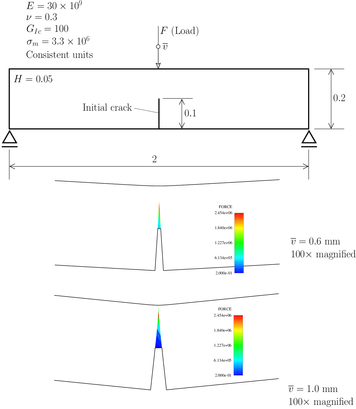
The classical three-point-bending test, represented in Figure 48↓ is employed here for verification. A constitutive law reproducing a mode I cohesive law:
E1 = E
E2 = E3 = 0
The purpose of this test is to assess the following required non-constitutive data:
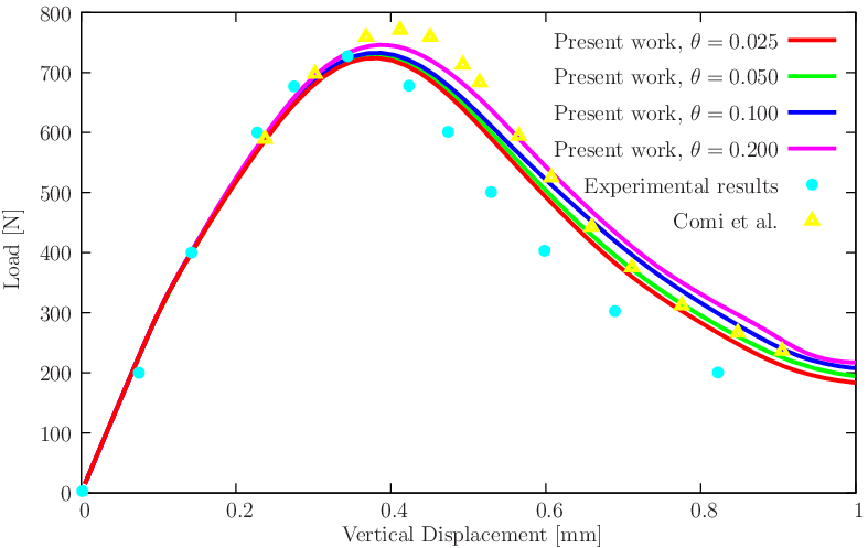
Effect of the non-dimensional characteristic length parameter θ (with values 0.025, 0.050, 0.100 and 0.200).
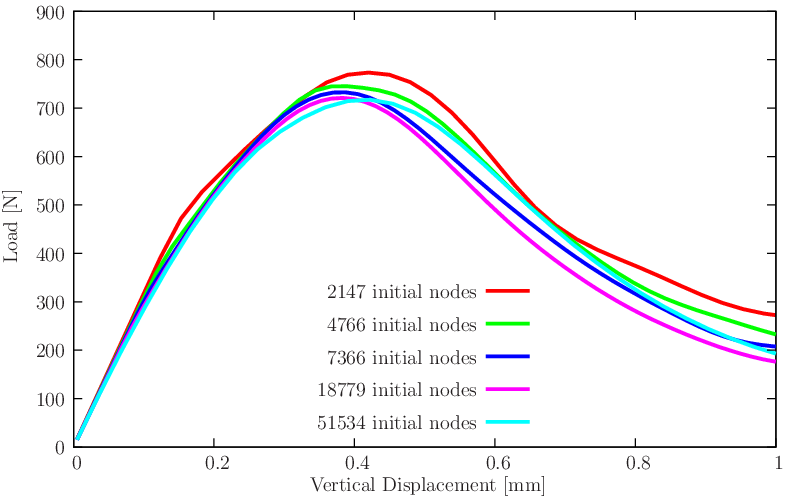
Effect of mesh size (free triangular meshes with 2147, 4766, 7366, 18779 and 51534 nodes).
Figure 48 Verification with the three-point-bending test: relevant data and forces in the cohesive region.
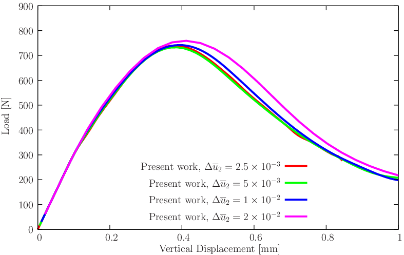
In Figure 48↑, we can also observe two steps with the injected softening elements, for v = 0.6 mm and v = 1 mm. Geometry is 100 × magnified. For comparison, we use both numerical and experimental results provided, respectively, by Claudia Comi [18] and co-workers (numerical results) and also the experimental data gathered by Alfaiate and co-workers [2]. Figure 49↓ shows the effect of band thickness (in the non-dimensional form θ) in the load/displacement results. Subsequent Figures 50↓ and 51↓ show the effect of the step and mesh size, respectively.
Figure 49 Effect of θ in the load/displacement results: Δu2 = 5 × 10 − 3, 14154 initial elements, 7366 initial nodes.
Figure 50 Effect of Δu2 in the load/displacement results: θ = 0.1, 14154 initial elements, 7366 initial nodes.
Figure 51 Effect of number of nodes in the load/displacement results: θ = 0.1, Δu2 = 5 × 10 − 3.
The conclusions that can be drawn from the inspection of Figures 49↑-51↑ are:
The effect of θ in the load/deflection results is observable, but somehow limited and in-line with the expectable accuracy for fracture problems.
The effect of step size is observable for large step sizes (in Figure 50↑) but subsequent decrease in step size becomes irrelevant.
Moderate mesh size dependence still exists, but not in a monotonous form, as observed in Figure 51↑.
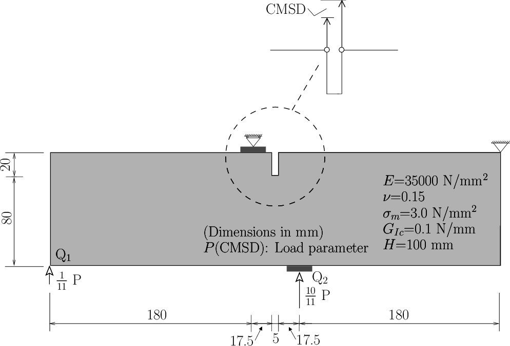
This version of the single-edge-notched beam problem was introduced by Schlangen (cf. [46]) and is now modeled. It consists of a pre-notched beam loaded in two points and supported in other two points. Figure 52↓ contains the relevant data for this problem. It is appropriate for the assessment of the injection method since the experimentally observed result is a curved crack emanating from the right corner of the notch. Curved cracks are difficult to reproduce with smeared models. Since \bmP cannot be monotonous when crack propagation occurs, a control equation is used, which increases the shear mouth relative displacement of the initial notch (cf. Figure 52↓). This is called crack mouth sliding displacement (CMSD) and is imposed at the global level.
Figure 52 Schlangen’s SEN specimen: relevant data.
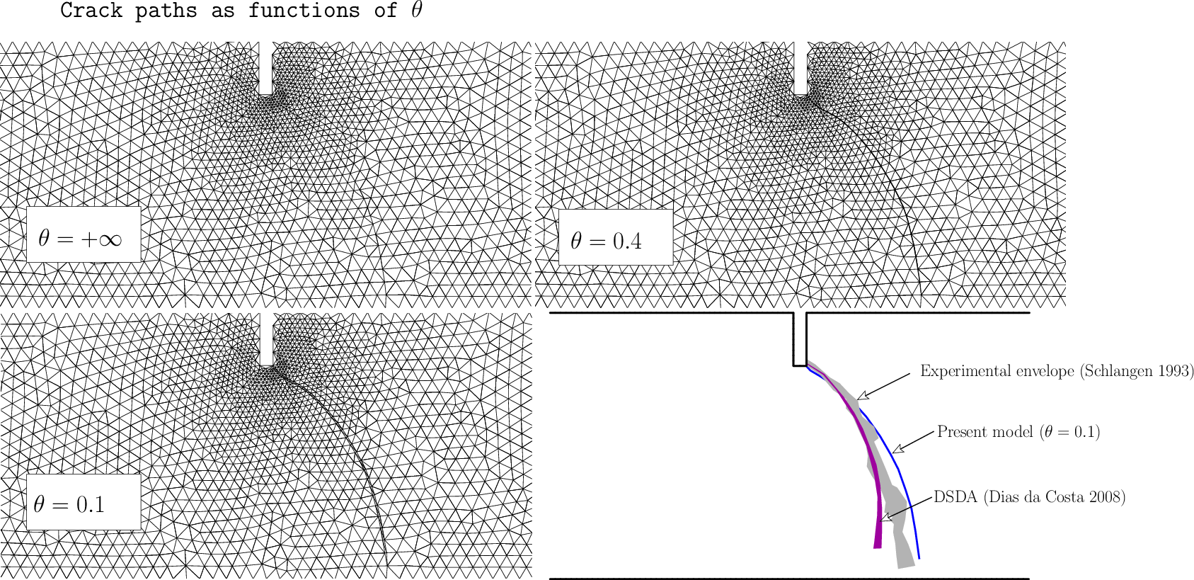
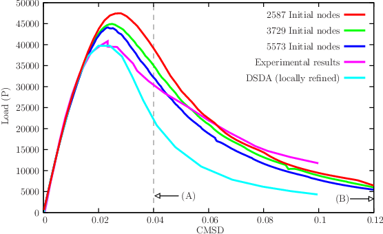
We test three triangular meshes containing 2587, 3729 and 5573 nodes. The resulting crack path is not far from the experimental envelope, as can be observed in Figure 53↓; even near the support the experimental observations are reasonably reproduced. A comparison with the experimental results and the DSDA method [2, 6], along with a study of mesh size influence is performed. As can be observed in Figure 55↓, after the peak load is reached, the numerical results are more brittle than the experimental results. According to Alfaiate, Wells and Sluys [3], this is due to the fact that an isotropic mode-I traction-jump law is used. Since crack paths are nearly insensitive to the value of θ, we fix the value θ = 0.2 for the mesh size effect study.
Figure 53 Schlangen’s SEN specimen: crack paths comparison. Crack paths from Schangen [46] are shown.
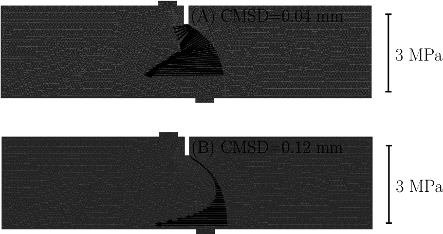
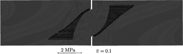
Figure 54 Cohesive vector tails for two distinct values of CMSD (A and B). Finer mesh is adopted.
(a) CMSD/load results
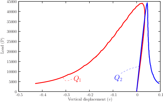
(b) Load (P) versus vertical displacement of points Q1 and Q2 . Results for the finer mesh are shown.
Figure 55 CMSD/load results, compared with the experimental results by Schlangen [46] and the DSDA technique [104].
4.3Cohesive crack growth in a four-point bending concrete beam
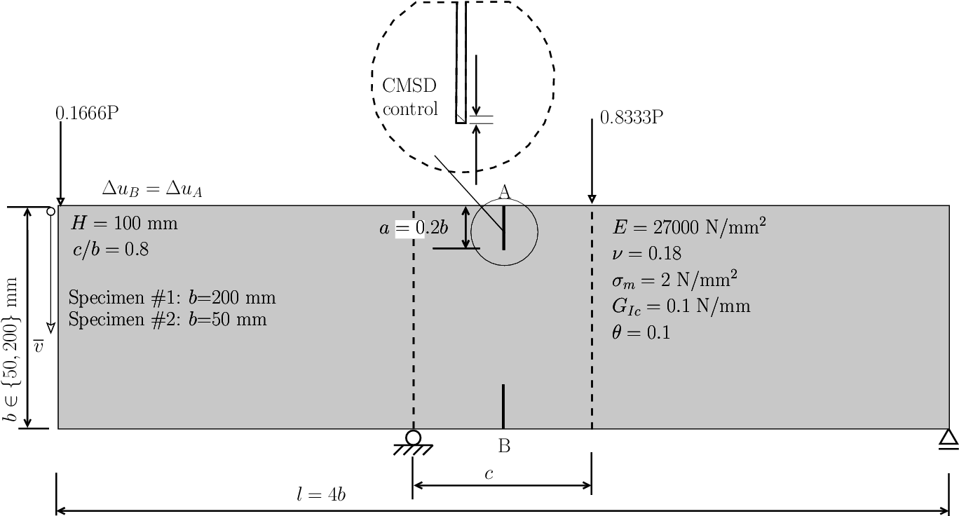
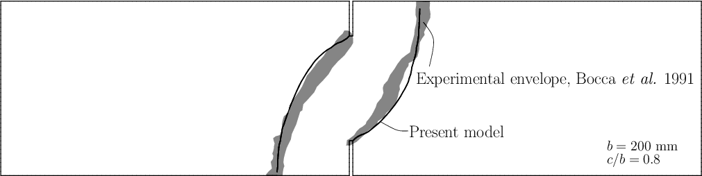
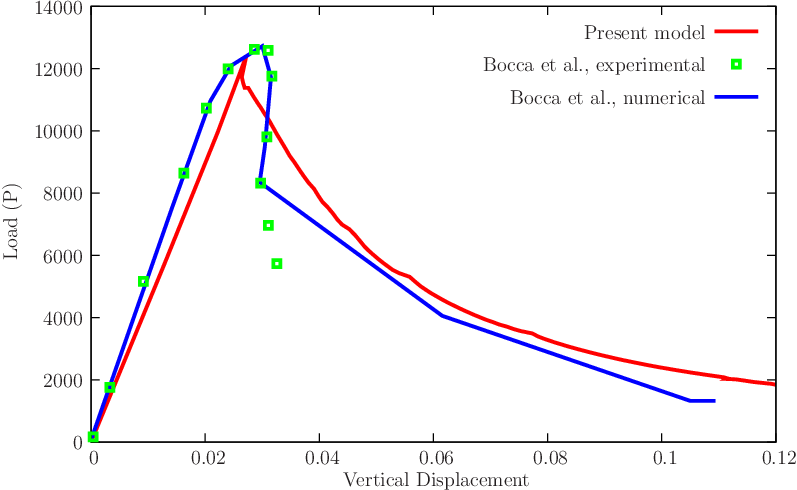
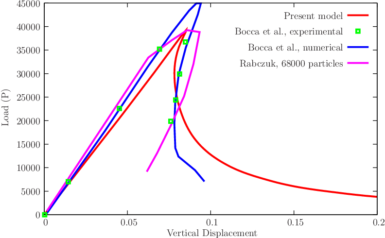
The bi-notched concrete beam proposed by Bocca et al.[15] is tested. The beam is simply supported in two points and subjected to two point loads. The effect of beam size in brittleness is assessed by using two different specimen dimensions. The corresponding experimental setting is described in detail in the original work [15]. From the set of specimens studied by Bocca et al. we retain the specimens, both with c ⁄ b = 0.8: one with b = 50 and another with b = 200 mm. These have reported experimental measurements in [15]. We are also concerned with the crack paths that were reported in [15]. Using the well-known cracking particle method, Rabczuk and Belytschko [42] obtained very good results for the crack path prediction, although with a slightly higher load than the experimental one. However, with the particle methods, there is an ambiguity in assigning the support dimension for the crack region. We use a single uniform initial mesh, with 7488 nodes and 14536 triangular elements. All relevant data is shown in Figure 56↓. For anti-symmetry reasons, we force the same mouth horizontal displacement at the edge of notches A and B: ΔuB = ΔuA. It has been debated if quasi-static simulations allow propagation of more than one crack (concerning this topic, see the excellent thesis by Chaves [110]), and the imposition of same relative displacement forces both cracks to evolve simultaneously. We obtain an excellent agreement with the experimental crack paths, as shown in Figure 57↓. The relatively wide spread of experimental crack paths is typical and is a consequence of the use of 6 specimens of reference [15]. Experimentally, some residual crack evolution in the opposite direction of the final path was observed and we also obtained that effect. Load-displacement results are shown in Figure 58↓ where a comparison with the measurements of Bocca et al.[15] and the cracking particle method of Rabczuk and Belytschko [42] is made. For the smaller specimen there is a somehow longer and lower curve than the observed one.
Figure 56 Four-point bending of a concrete beam: geometry, boundary conditions, multiple point constraints (ΔuB = ΔuA) and material properties. Also shown is the final deformed mesh 10 × magnified with the attached cohesive stress vectors.
Figure 57 Four-point bending of a concrete beam: crack paths compared with the envelope of experimental results by Bocca, Carpintieri and Valente [15].
(a) b = 50 mm
(b) b = 200 mm
Figure 58 Load-displacement results, compared with the results of Bocca et al. [15]and the cracking particle method of Rabczuk and Belytschko [42] (for the case b = 200 mm) with their 68000 particle analysis.
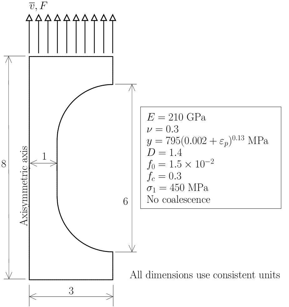
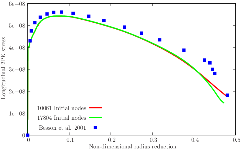
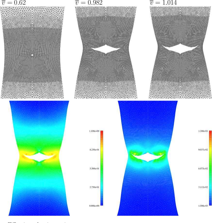
A tension test producing cup and cone fracture was described by Besson [14] and is here reproduced. We include explicit crack propagation by element injection subsequently to the satisfaction of f ≥ ff. Figure 59↓ shows relevant data for this problem. The stress/displacement results are compared with results obtained by Besson et al.[14]. We are also concerned with the cup and cone formation, which requires a sufficiently refined mesh and elongated elements in the radial direction. Figure 61↓ shows the crack formed in the necking region and propagating toward the outer surface, forming the cup and cone. This type of result, combining the localization in ductile materials and a physically meaningful ductile crack formation is very rare in the literature. In addition, robustness is an advantage when compared with GFEM/XFEM. The stress/displacement results are compared with results obtained by Besson et al.[14]. Crack path formation is compared between the two meshes in Figure 62↓. Some differences can be observed in the crack path, but these results are in-line with what is expected from crack propagation analysis with ductile materials.
Figure 59 Besson cylindrical specimen modeled with axisymmetric elements. Relevant data (see also [14]).
Figure 60 Besson cylindrical specimen: second Piola-Kirchhoff stress vs. radial reduction, compared with the results of Besson et al.[14].
Figure 61 Besson cylindrical specimen: cup and cone formation and corresponding contour plots (f and εp).
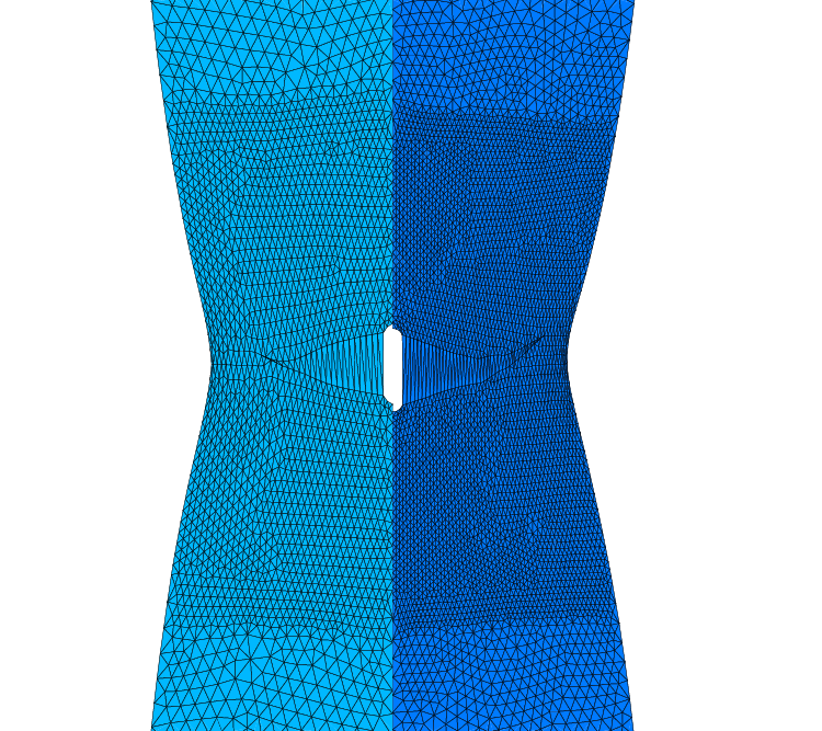
Figure 62 Crack path formation: comparison between 10061 and 17804 initial nodes.
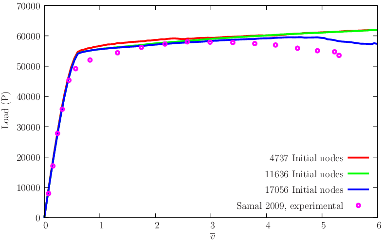
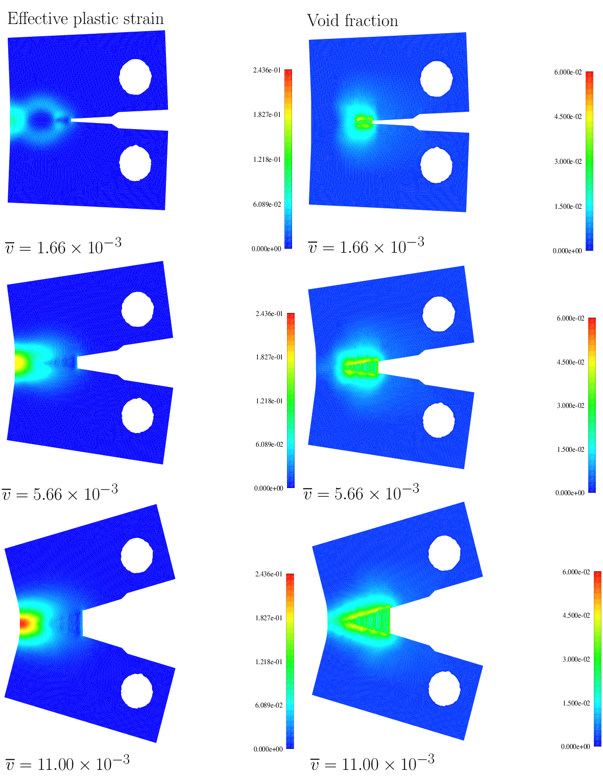
The compact tension specimen described by Samal et al.[43] is reproduced. In that paper, the Rousselier yield function was adopted to model ductile fracture of a pre-cracked (a0 = 0.0161 m) specimen. Experimental results were also reported. The Authors used a gradient model to attenuate the mesh dependence (equivalent to the one by Areias et al.[8]). Relevant data for this test is shown in Figure 63↓. Here, the initial crack is explicitly represented (which was not in the original paper). Hardening law is inserted as a set of ordered pairs, as shown in Table 1↓. We monitor the force F as a function of the imposed displacement v and compare with the experimental results reported in Samal’s paper. This comparison is presented in Figure 64↓ where good agreement can be observed, despite the slightly higher values of reaction obtained here. Note that higher numerical values were also reported by Samal et al.[43]. A sequence of contour plots for the void fraction and effective plastic strain is shown in Figure 65↓. Very high deformations are possible without convergence problems.
Figure 63 Compact tension specimen. Lengths given in meters. The hardening function is provided in [43].
Table 1 Hardening law used in the compact tension specimen (Figure 63↑).
εp
y [MPa]
0
405
0.0568
569
0.0710
584
0.0994
621
0.1207
634
0.1917
675
0.2864
721
0.5089
796
0.8260
881
1.1030
935
Figure 64 Compact tension specimen: comparison between experimental (reported in [43]) and numerical results for three different initial meshes.
Figure 65 Compact tension specimen (cf. [43]): sequence of effective plastic strain and void fraction contour plots.
References
[1] Abaqus/Standard Example Problems Manual, Volumes I and II. 2008.
[2] J. Alfaiate, A. Simone, L.J. Sluys. A new approach to strong embedded discontinuities. Computational Modelling of Concrete Structures, EURO-C 2003, 2003.
[3] J. Alfaiate, G.N. Wells, L.J. Sluys. On the use of embedded discontinuity elements with crack path continuity for mode-I and mixed-mode fracture. EFM, 69:661-686, 2002.
[4] U. Andelfinger, E. Ramm. EAS-elements for two-dimensional, three-dimensional, plate and shell structures and their equivalence to HR-elements. IJNME, 36:1311-1337, 1993.
[5] P. Areias, T. Belytschko. Non-linear analysis of shells with arbitrary evolving cracks using XFEM. IJNME, 62:384-415, 2005.
[6] P. Areias, J.M.A. César de Sá, C.A. Conceição António, J.A.S.A.O. Carneiro, V.M.P. Teixeira. Strong displacement discontinuities and Lagrange multipliers in the analysis of finite displacement fracture problems. CM, 35:54-71, 2004.
[7] P. Areias, J.M.A. César de Sá, C.A. Conceição António, A.A. Fernandes. Analysis of 3D problems using a new enhanced strain hexahedral element. IJNME, 58:1637-1682, 2003.
[8] P. Areias, J.M.A. César de Sá, Conceição António. A gradient model for finite strain elastoplasticity coupled with damage. FEAD, 39:1191-1235, 2003.
[9] P. Areias, D. Dias-da-Costa, E.B. Pires, J. Infante Barbosa. A new semi-implicit formulation for multiple-surface flow rules in multiplicative plasticity. CM, 49:545-564, 2012.
[10] P. Areias, J.-H. Song, T. Belytschko. A finite-strain quadrilateral shell element based on discrete Kirchhoff-Love constraints. IJNME, 64:1166-1206, 2005.
[11] Y. Basar, Y. Ding. Finite rotation shell elements for the analysis of finite rotation shell problems. IJNME, 34:165-169, 1992.
[12] K.-J. Bathe, E.N. Dvorkin. A formulation of general shell elements-the use of mixed interpolation of tensorial components. IJNME, 22:697-722, 1986.
[13] T. Belytschko, B.L. Wong. Assumed strain stabilization procedure for the 9-node Lagrance shell element. IJNME, 28:385-414, 1989.
[14] J. Besson, D. Steglich, W. Brocks. Modeling of crack growth in round bars and plane strain specimens. IJSS, 38:8259-8284, 2001.
[15] P. Bocca, A. Carpinteri, S. Valente. Mixed mode fracture of concrete. IJSS, 27(9):1139-1153, 1991.
[16] S. Cen, X.-M. Chen, X.-R. Fu. Quadrilateral membrane element family formulated by the quadrilateral area coordinate method. CMAME, 196:4337-4353, 2007.
[17] J.M.A. César de Sá, P. Areias, R.M. Natal Jorge. Quadrilateral elements for the solution of elasto-plastic finite strain problems. IJNME, 51:883-917, 2001.
[18] C. Comi, L. Driemeier. Material Instabilities in Solids. John Wiley and Sons, 1998.
[19] M.A. Crisfield, G.F. Moita, G. Jelenić, L.P.R. Lyons. Enhanced lower-order element formulation for large strains. CM, 17:62-73, 1995.
[20] E.N. Dvorkin, K.J. Bathe. A continuum mechanics based four node shell element for general nonlinear analysis. EC, 1:77-88, 1984.
[21] R. Eberlein, P. Wriggers. Finite element concepts for finite elastoplastic strains and isotropic stress response in shells: Theoretical and computational analysis.CMAME, 171:243-279, 1999.
[22] A. Eriksson, C. Pacoste. Element formulation and numerical techniques for stability problems in shells. CMAME, 191:3775-3810, 2002.
[24] S. Glaser, F. Armero. On the formulation of enhanced strain finite elements in finite deformations. EC, 14(7):759-791, 1997.
[25] S. Hartmann, J. Oliver, R. Weyler, J.C. Cante, J.A. Hernández. A contact domain method for large deformation frictional contact problems. Part 2: Numerical aspects. CMAME, 198:2607-2631, 2009.
[26] R. Hauptmann, S. Doll, M. Harnau, K. Schweizerhof. Solid-shell elements with linear and quadratic shape functions at large deformations with near incompressible materials. CS, 79:1671-1685, 2001.
[27] T.J.R. Hughes. The finite element method. Dover Publications, 2000. Reprint of Prentice-Hall edition, 1987.
[28] S. Klinkel, F. Gruttmann, W. Wagner. A mixed shell formulation accounting for thickness strains and finite strain 3D material models. IJNME, 74:945-970, 2008.
[29] J. Korelc, P. Wriggers. Improved enhanced strain four-node element with Taylor expansion of the shape functions. IJNME, 40:407-421, 1997.
[30] T.A. Laursen. Computational contact and impact mechanics. Fundamentals of modeling interfacial phenomena in nonlinear finite element analysis. Springer, 2002.
[31] T.A. Laursen. Computational contact and impact mechanics. Fundamentals of modeling interfacial phenomena in nonlinear finite element analysis. Springer, 2002.
[32] W.K. Liu, Y. Guo, T. Belytschko. A multiple-quadrature eight-node hexahedral finite element for large deformation elastoplastic analysis. CMAME, 154:69-132, 1998.
[34] F. Ma, X. Deng, M.A. Sutton, J.C. Newman. Mixed-mode crack behavior. ASTM American Society for Testing and Materials, 1999.
[35] R.H. MacNeal, R.L. Harder. A proposed standard set of problems to test finite element accuracy. FEAD, 1:1-20, 1985.
[36] C.M. Muscat-Fenech, A.G. Atkins. Out-of-plane stretching and tearing fracture in ductile sheet materials. International Journal of Fracture, 84:297-306, 1997.
[37] T.H.H Pian, K. Sumihara. Rational approach for assumed stress finite elements. IJNME, 20:1685-1695, 1984.
[38] R. Piltner, R.L. Taylor. A quadrilateral mixed finite element with two enhanced strain modes. IJNME, 38:1783-1808, 1995.
[39] G. Prathap, V. Senthilkumar. Making sense of the quadrilateral area coordinate membrane elements. CMAME, 197:4379-4382, 2008.
[40] M.A. Puso, T.A. Laursen. A mortar segment-to-segment contact method for large deformation solid mechanics. CMAME, 193:601-629, 2004.
[41] M.A. Puso, T.A. Laursen. A mortar segment-to-segment frictional contact method for large deformations. CMAME, 193:4891-4913, 2004.
[42] T. Rabczuk, T. Belytschko. Cracking particles: a simplified meshfree method for arbitrary evolving cracks. IJNME, 61:2316-2343, 2004.
[43] M.K. Samal, M. Seidenfuss, E. Roos. A new mesh-independent Rousselier's damage model: Finite element implementation and experimental verification. IJMS, 51:619-630, 2009.
[44] C. Sansour, J. Bocko. On hybrid stress, hybrid strain and enhanced strain finite element formulations for a geometrically exact shell theory with drilling degrees of freedom. IJNME, 43(1):175—192, 1998.
[45] C. Sansour, F.G. Kollmann. Families of 4-node and 9-node finite elements for a finite deformation shell theory. An assessment of hybrid stress, hybrid strain and enhanced strain elements. CM, 24:435-447, 2000.
[46] E. Schlangen. Experimental and numerical analysis of fracture processes in concrete. 1993.
[47] M. Schonauer, E.A. de Souza Neto, D.R.J. Owen. Hencky tensor based enhanced large strain element for elasto-plastic analysis. Computational Plasticity: Fundamentals and Applications, 1:333-348, 1995.
[48] H. Schoop, J. Hornig, T. Wenzel. Remarks on Raasch's hook. TM, 4(22):259-270, 2002.
[49] J.C. Simo, F. Armero, R.L. Taylor. Improved versions of assumed strain tri-linear elements for 3D finite deformation problems. CMAME, 110:359-386, 1993.
[50] J.C. Simo, F. Armero. Geometrically non-linear enhanced strain mixed methods and the method of incompatible modes. IJNME, 33:1413-1449, 1992.
[51] J.C. Simo, D.D. Fox, M.S. Rifai. Geometrically exact stress resultant shell models: Formulation and computational aspects of the nonlinear theory. Analytical and Computational Models of Shells, 3:161-190, 1989.
[52] J.C. Simo, M.S. Rifai. A class of mixed assumed strain methods and the method of incompatible modes. IJNME, 29:1595-1638, 1990.
[53] J.C. Simo, R.L. Taylor, K.S. Pister. Variational and projection methods for the volume constraint in finite deformation elasto-plasticity. CMAME, 51:177-208, 1985.
[54] K.Y. Sze, Y.S. Kim, A.K. Soh. A hybrid stress quadrilateral shell element with full rotational DOFS. IJNME, 40:1785-1800, 1997.
[55] I. Temizer. A mixed formulation of mortar-based frictionless contact. CMAME, 223-224:173-185, 2012.
[56] W. Wagner, S. Klinkel, F. Gruttmann. Elastic and plastic analysis of thin-walled structures using improved hexahedral elements. CS, 80:857-869, 2002.
[57] B. Yang, T.A. Laursen, X. Meng. Two dimensional mortar contact methods for large deformation frictional sliding. IJNME, 62:1183-1225, 2005.
[58] O.C. Zienkiewicz, R.L. Taylor. The finite element method. Butterworth Heinemann, 2000.